
Font size
 Worksheets
Introduction to MS Excel
Total questions: 25
Worksheet time: 15mins
Write your name and section.
To what category of software does MS Excel belong to?
Drawing
Database
Spreadsheet
Operating System
A spreadsheet is a large sheet of paper with columns and rows, and was originally used in accounting to organize data about business transactions.
True
False
What is Excel primarily used for?
Word processing
Graphic design
Email communication
Data analysis and manipulation
Which of the following is a collection of worksheets within a single file in Excel?
worksheet
workbook
spreadsheet
datasheet
What is the intersection of a column and a row in Excel called?
Cell
Worksheet
Workbook
Formula
In Excel, what is the reference for a single cell called?
Cell address
Cell range
Formula bar
Name Box
Which part of the Excel window displays the contents of the active cell?
Title Bar
Name Box
Formula Bar
Status Bar
What is a group of cells in Excel that are close together and can be manipulated together called?
Cell address
cell range
cell cloud
cell colony
Each column in a worksheet is identified by a __________.
number
letter
a letter and a number
a special character
___are horizontal and are identified by numbers.
columns
rows
address
range
AA3 is an example of a cell address.
True
False
64B is an example of a cell address
True
False
A cell has a unique address consisting of a column letter and row number.
binary letter and number
column number and row letter
column letter and row number
random letter and number
You can visually tell the current active cell in a worksheet by its __________.
different color
arrow
bigger dimension
thick "border"
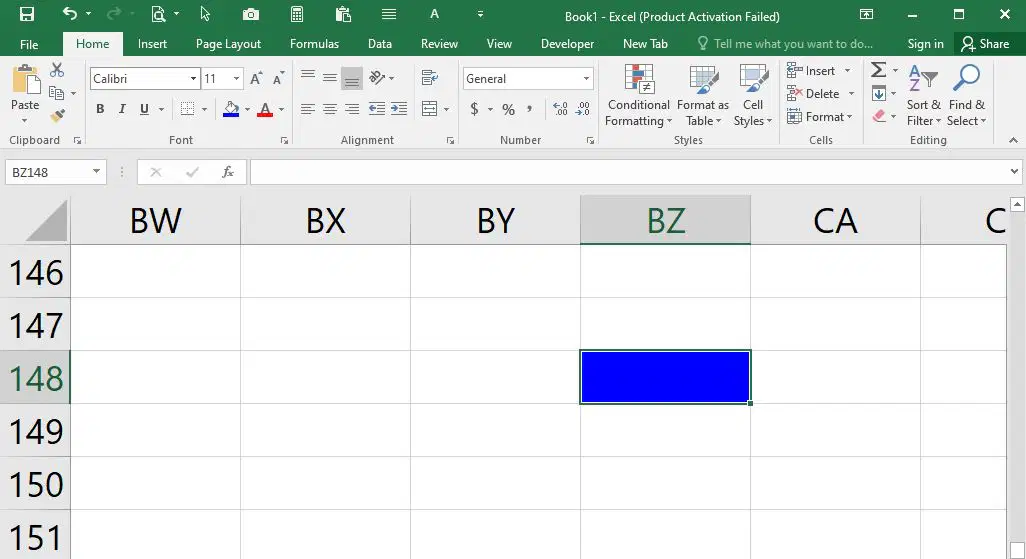
What is the cell address of the cell with blue highlight in the picture?
(a)

What is the cell address of the range selected in the picture?
(a)
What type of information can be entered in a worksheet?
words, sentences, and paragraphs
labels, constants, and formulas
records, fields, and database
images, pictures, and illustrations
Labels, values, or formulas entered in a cell is also displayed in the __________ where you can also edit it.
formula bar
status bar
name box
title bar
Which of the following is used to organize and analyze data in Excel?
Formula
Conditional Formatting
Sorting
AutoFill
Which Excel feature is used to create a series of data such as numbers or dates?
Formula
Conditional Formatting
Sorting
AutoFill
Which Excel feature allows you to apply different formatting to a cell or range based on certain conditions?
Formula
Conditional Formatting
Sorting
AutoFill
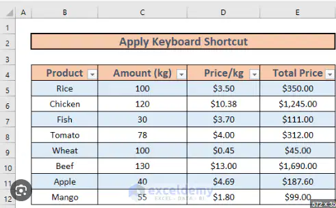
Reorder the following to make it the correct sequence of steps to sort the data in the picture in descending order in terms of total price.
A. Check the "My Data has Headers" checkbox.
B. Sort On: "values", Order: "Largest to Smallest"
C. Select cell range B4:E12.
D. In the "Sort by" portion, click the arrow down and then select "Total Price".
E. In the Home Menu, click Sort & Filter, and then select Custom Sort.
F. Click OK to sort data
CEADBF
ABCDEF
BEDCAF
DABCEF

If we apply Sort by Remarks (Z to A), then by Names (A to Z) to the table on the picture, which of the following table will be the result?


I want to highlight the average of the students who failed with light pink fill and red font. Which of the following steps is the correct order of doing this?
Select the table --> In the Home Tab, select Conditional Formatting --> Select Highlight Cells Rules --> Select Less Than --> Type 75 in the dialog box --> Select light pink fill and red font --> Click Okay
Select the table --> In the Home Tab, select Conditional Formatting --> Select Highlight Cells Rules --> Select Equal to --> Type 75 in the dialog box --> Select light pink fill and red font --> Click Okay
Select the table --> In the Home Tab, select Conditional Formatting --> Select Highlight Cells Rules --> Select Greater Than --> Type 75 in the dialog box --> Select light pink fill and red font --> Click Okay
Manually check each data one by one and highlight the average of the students who failed.