An analyst estimates a model and finds that the Breusch-Pagan test statistic is 5.92 with a critical value of 3.84 at the 5% level. What is the correct conclusion?

In a multiple regression with 150 observations and 12 predictors, which of the following is most likely true?

Which of the following situations most clearly indicates multicollinearity?

An analyst suspects higher-order serial correlation (beyond first order) in the residuals of a time-series regression. Which approach is most appropriate?

In probit and logit models, why can’t the estimated coefficients be interpreted as direct changes in probability?

A researcher wants to model the likelihood that a firm engages in ESG reporting (1 = reports, 0 = does not report). Which of the following is the most appropriate justification for using a probit or logit model instead of a linear probability model (LPM)?

Gary Hansen is a securities analyst for a mutual fund specialising in small-capitalisation growth stocks. The fund regularly invests in initial public offerings (IPOs). If the fund subscribes to an offer, it is allocated shares at the offer price. Hansen notes that IPOs frequently are underpriced, and the price rises when open market trading begins. The initial return for an IPO is calculated as the change in price on the first day of trading divided by the offer price. Hansen is developing a regression model to predict the initial return for IPOs. Based on past research, he selects the following independent variables to predict IPO initial returns:

• Underwriter rank = 1–10, where 10 is the highest rank

• Pre-offer price adjustment (a) = (Offer price – Initial filing price) / Initial filing price

• Offer size ($ millions) = Shares sold × Offer price

• Fraction retained (a) = Fraction of total company shares retained by insiders (expressed as a decimal)

Hansen collects a sample of 1,725 recent IPOs for his regression model. Regression results appear in Exhibit 1, and ANOVA results appear in Exhibit 2.

Hansen wants to use the regression results to predict the initial return for an upcoming IPO. The upcoming IPO has the following characteristics:

• Underwriter rank = 6

• Pre-offer price adjustment = 0.04

• Offer size = $40 million

• Fraction retained = 0.70

Because he notes that the pre-offer price adjustment appears to have an important effect on initial return, Hansen wants to construct a 95 per cent confidence interval for the coefficient on this variable. He also believes that for each 1 per cent increase in pre-offer price adjustment, the initial return will increase by less than 0.5 per cent, holding other variables constant. Hansen wishes to test this hypothesis at the 0.05 level of significance. (The two-tailed critical value at 5% significance level is 1.96, while the 5% one-tailed critical value is 1.65).

Before applying his model, Hansen asks a colleague, Phil Chang, to review its specification and results. After examining the model, Chang concludes that the model suffers from a problem: conditional heteroskedasticity. Chang makes the following statement:

Statement 1: Conditional heteroskedasticity will result in consistent coefficient estimates, but both the t-statistics and F-statistic will be biased, resulting in false inferences.

Gary Hansen Case Study, Q1

Based on Hansen’s regression, the predicted initial return for the upcoming IPO is closest to:

Gary Hansen Case Study, Q2

The 95 per cent confidence interval for the regression coefficient for the pre-offer price adjustment is closest to:

Gary Hansen Case Study, Q3

The most appropriate null hypothesis and the most appropriate conclusion regarding Hansen’s belief about the magnitude of the initial return relative to that of the pre-offer price adjustment (reflected by the coefficient, 0.05 level of significance) are:

Gary Hansen Case Study, Q4

The most appropriate interpretation of the multiple R-squared for Hansen’s model is that:

Gary Hansen Case Study, Q5

Is Chang’s Statement 1 correct?

Info for Yacktman Case Study

Evaluating the Performance of the Yacktman Focused Fund

You are an individual investor evaluating whether to allocate capital to the Yacktman Focused Fund. To assess the fund’s performance, you estimate the following Fama and French (1993) three-factor model using 180 monthly observations of the fund’s excess returns and risk factor data:

ExcR_t = $$\alpha$$ + $$\beta$$ _MKTMKT_t + $$\beta$$ _SMBSMB_t + $$\beta$$ _HMLHML_t + $$\epsilon$$ _t

MKT: is the excess return on the market in month  (the market return minus the risk-free rate in month t).

• SMB(Small Minus Big): is the average return on small stock portfolios minus the average return on big stock portfolios in month t. 

• HML (High Minus Low): is the average return on value (high book-to-market) stock portfolios minus the average return on growth (low book-to-market) stock portfolios in month t.

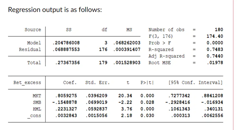
Regression output is as follows:

Yacktman Case Study, Q1

Based on the regression output, which of the following is the most accurate interpretation of the factor loadings?

Yacktman Case Study, Q2

The alpha, $$\alpha$$ in the above regression captures the average risk-adjusted return (known as abnormal return or return beyond risk exposures) of the fund. Using a 5% significance level (two-tailed), does the fund manager generate statistically significant abnormal performance? 

Critical t-value (df = 176): 1.97

Yacktman Case Study, Q3

You test whether the coefficient on the market factor is equal to 1:

H₀ : $$\beta$$ _MKT = 1

Given:

t = $$\frac{0.8059-1}{0.0396}$$ = -4.90

and the Critical t-value at 5% significance level and 176 df is 1.97.

What is the correct inference?

Yacktman Case Study, Q4

You suspect model misspecification and run a Breusch–Pagan test using squared residuals. The auxiliary regression produces R² = 0.0605, and:

LM = nR² = 180 x 0.0605 = 10.89

The critical chi-square at 5% is $$\chi^2$$ (3, 0.95) = 7.8147279

Which conclusion is most appropriate?

Yacktman Case Study, Q5

To test for serial correlation, you run a Breusch–Godfrey LM test (1 lag). The auxiliary regression produces: 

R² = 0.042, LM = nR² = 180 x 0.042 = 7.56

The 5% critical value from the chi-square distribution (1 df) is 3.84.

What is the correct conclusion?

An analyst examines whether firm size explains variation in earnings volatility using a sample of 150 firms. After estimating the regression, the analyst conducts a Breusch–Pagan test for heteroskedasticity by regressing the squared residuals on firm size. The auxiliary regression reports:

R² = 0.012

The Breusch–Pagan test statistic is computed as:

LM = n x R² = 150 x 0.012 = 1.80

At the 5% significance level, the critical value from the chi-squared distribution with 1 degree of freedom is approximately 3.84. What is the correct inference?

An economist analyses monthly housing price inflation using a regression model that includes interest rates, income growth, and supply indicators. To test for first-order serial correlation in the residuals, the economist performs a Breusch–Godfrey (BG) test. The auxiliary regression of residuals on their lagged value and the original regressors yields:

R² = 0.027

The BG test statistic is computed as:

LM = n x R² = 200 x 0.027 = 5.40

At the 5% significance level, the critical value from the chi-squared distribution with 1 degree of freedom is 3.84. What is the correct inference?

Which of the following statements best describes panel data?