
 Worksheets
AP Stats Unit 3 Practice Test
Total questions: 26
Worksheet time: 14mins
Simone wanted to study how hydration levels change after different durations of running. She measured each participant’s hydration level (in liters) before running and then randomly assigned each participant to run for 0, 20, 40, or 60 minutes. After running, she recorded the participant’s change in hydration level.
The response variable is the participant’s hydration level before running and it is categorical.
The response variable is the participant’s hydration level before running and it is quantitative.
The response variable is the participant’s change in hydration level and it is categorical.
The response variable is the participant’s change in hydration level and it is quantitative.
The response variable is the number of minutes of running and it is quantitative.
The number of hours spent on homework and the hours of free time in a random sample of 13-year-olds was recorded. The value of the correlation coefficient was –0.50. In order to predict hours of free time based on the number of hours spent on homework, the least-squares regression line will be determined. Which of the following is an incorrect statement?
The slope of the least-squares regression line is negative.
Higher values for the number of hours spent on homework tend to be paired with lower values of hours of free time.
The strength of the association between hours of free time and hours of homework is moderate.
The least-squares regression line accounts for 25% of the variability in hours of free time.
The least-squares regression line captures 50% of the observed hours of free time.
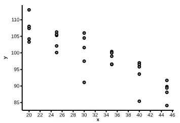
Which of the following values is closest to the correlation between the two variables shown in the scatterplot?
-1
-0.8
-0.3
0.4
0.8
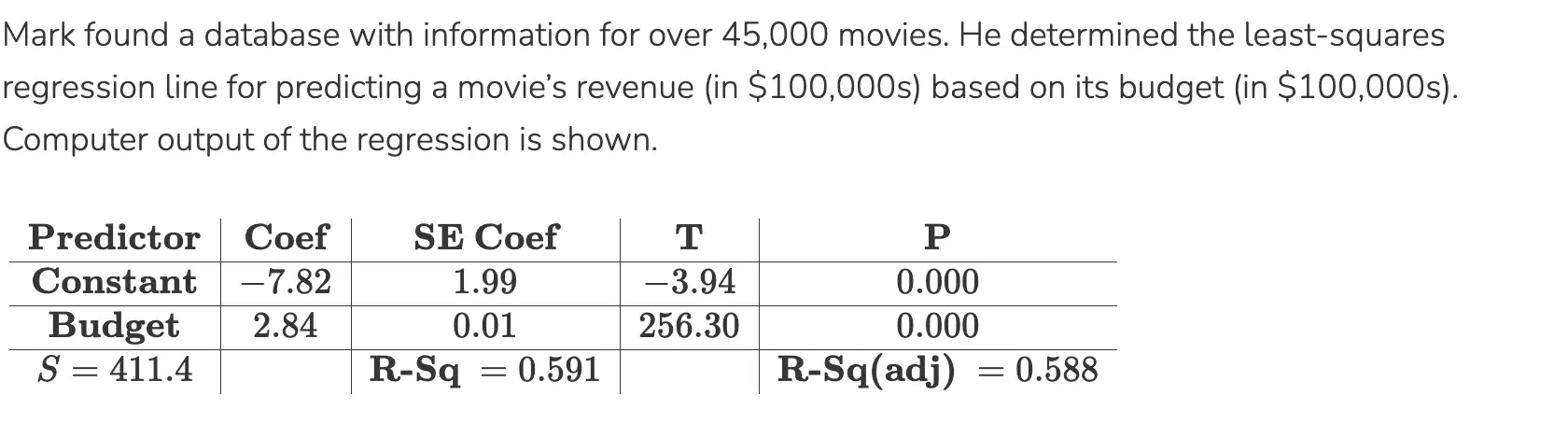
Which of the following is the equation of the least-squares regression line?
Revenue = -7.82 + 2.84 (Budget)
Budget = -7.82 + 2.84 (Revenue)
Revenue = 2.84 - 7.82 (Budget)
Budget = 2.84 - 7.82 (Revenue)
Revenue = -7.82 + 411.4 (Budget)
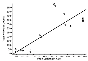
For a project in his statistics class, Caden took a random sample of 10 entries from Wikipedia.com and recorded the length of the page (in kilobytes) and the number of views (in 1000s) the page had in the past 30 days. He determined the least-squares regression line using the page length to predict the number of page views. A scatterplot and least-squares regression line for these data are shown. Five of the observations are labeled A through E. Which observation has the largest absolute value of the residual?
A
B
C
D
E
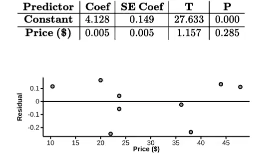
Kim recorded the price (in dollars) and customer rating of nine pairs of women’s shoes. The data were used to create the residual plot and regression output shown. Which of the following is closest to the actual customer rating of the pair of shoes that has a price of $21.99?
4
4.1
4.2
4.3
4.5
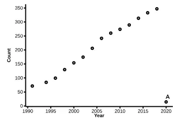
An analyst for a study abroad program found data on the count of students (in thousands) attending colleges outside their home country and the academic year. The scatterplot shows the relationship between these two variables. If the point labeled A is removed, which of the following statements would be true?
The slope of the least-squares regression line would increase and the strength of the association would increase.
The slope of the least-squares regression line would increase and the strength of the association would decrease.
The slope of the least-squares regression line would increase and the strength of the association would remain the same.
The slope of the least-squares regression line would decrease and the strength of the association would increase.
The slope of the least-squares regression line would decrease and the strength of the association would decrease.
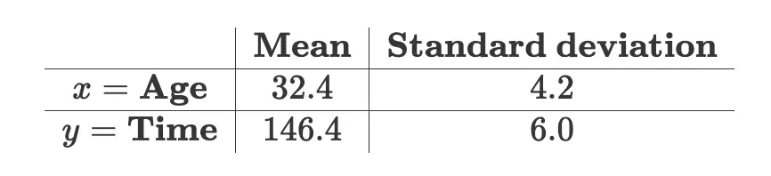
The table shows summary statistics for the times (in minutes) and ages (in years) of females with the fastest time at the Boston Marathon in each of the the past 10 years. The correlation between time and age was found to be r = -0.05. Which of the following is the approximate equation of the least-squares regression line for predicting y = time based on x = age?
A) ŷ = 27.28 - 0.035x
B) ŷ = 144.1 - 0.071x
C) ŷ = 148.71 - 0.071x
D) ŷ = 145.27 - 0.035x
E) ŷ = 100.11 - 1.430x

Psychologists were interested in how sound levels distract individuals in studying environments. They randomly assigned subjects to various decibel levels from 40 dB (quiet conversation) to 80 dB (loud music). Subjects were asked to rate how much the sound would distract them from studying on a numerical scale, from 1 to 10, where 1 represents "no distraction" and 10 represents "extreme distraction." A scatterplot (not shown) revealed a curved pattern, so the psychologists took the natural logarithm of the subjects’ ratings. The regression output shows the results for predicting ln(ratings) from the decibel level.
Which of the following is closest to the predicted rating for a subject who experienced a decibel level of 50?
0.51
1.66
1.98
3.91
0.054
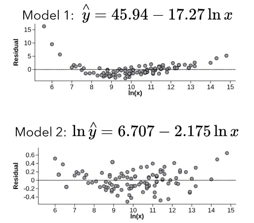
An observational study measured two quantitative variables, X and Y, for a random sample of 100 individuals. An analyst fit two different regression models, Model 1 and Model 2, to the data. The regression equation and residual plot for each model are shown below. Which of the following conclusions is correct?
Model 1 is appropriate, because the association between x and y is linear.
Model 1 is appropriate, because the association between ln(x) and y is linear.
Model 1 is appropriate, because the association between ln(x) and y is non-linear.
Model 2 is appropriate, because the association between x and y is linear.
Model 2 is appropriate, because the association between ln(x) and ln(y) is linear.
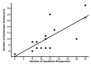
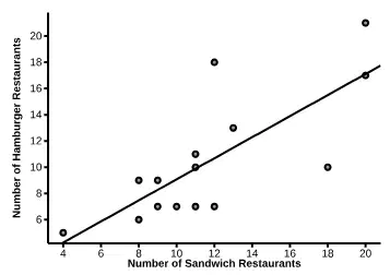
In order to describe the relationship between the two variables, we would say:
There is a
(a) , (b) , (c) relationship between the number of sandwich restaurants and the number of restaurants in town.
Interpret the
y-intercept of the least-squares regression line in context.
In a town with 0 sandwich restaurants, the predicted number of hamburger restaurants is 1.0421.
In a town with 1 sandwich restaurants, the predicted number of hamburger restaurants is 1.0421.
In a town with 1.0421 sandwich restaurants, the predicted number of hamburger restaurants is 0.
In a town with 0 sandwich restaurants, the predicted number of hamburger restaurants is 4.
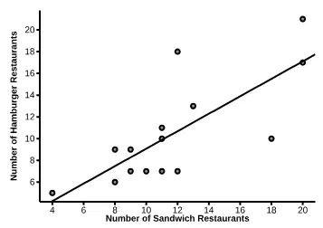
A random sample of 15 different towns in Michigan was selected. The scatterplot shows the relationship between the number of sandwich restaurants and the number of hamburger restaurants for each town. The least-squares regression line is ŷ = 1.0421 + 0.8032x, where y = number of hamburger restaurants in the town and x = number of sandwich restaurants in the town. Use the least-squares regression line to predict the number of hamburger restaurants in a town with 18 sandwich restaurants.
The predicted number of hamburger restaurants is approximately 15.5.
The predicted number of hamburger restaurants is approximately 12.4.
The predicted number of hamburger restaurants is approximately 20.1.
The predicted number of hamburger restaurants is approximately 10.2.
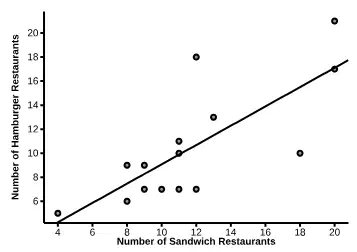
The town with 18 sandwich shop has 10 hamburger restaurants. Calculate and interpret the residual.
The residual is -5.5, meaning the actual number of hamburger restaurants is 5.5 less than predicted by the regression line.
The residual is 5.5, meaning the actual number of hamburger restaurants is 5.5 more than predicted by the regression line.
The residual is 4.5, meaning the actual number of hamburger restaurants is 4.5 more than predicted by the regression line.
The residual is -4.5, meaning the actual number of hamburger restaurants is 4.5 less than predicted by the regression line.
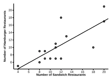
Can we conclude that an increase in the number of sandwich restaurants will cause an increase in the number of hamburger restaurants?
No, correlation does not imply causation.
Yes, an increase in sandwich restaurants will always cause an increase in hamburger restaurants.
Yes, because both serve similar food.
No, an increase in sandwich restaurants will decrease hamburger restaurants.
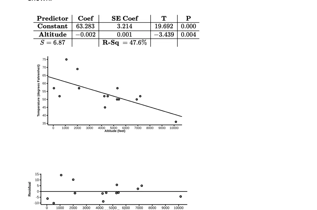
A linear model is appropriate for the data. Give two reasons to justify your answer.
Yes, because the scatterplot shows a linear trend, the residual plot shows a random scatter of residuals, and the correlation is moderately strong at r = -0.69.
No, because the data points are scattered randomly and show no pattern.
No, because the data shows a clear curve and not a straight line.
Yes, because the data points are clustered at one value and there is no pattern.
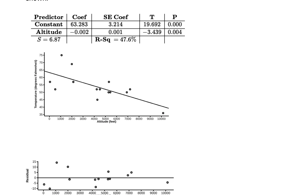
The slope of the least-squares regression line represents:
The predicted change in the response variable for each one-unit increase in the explanatory variable.
The value of the response variable when the explanatory variable is zero.
The strength of the linear relationship between two variables.
The average of the explanatory variable.
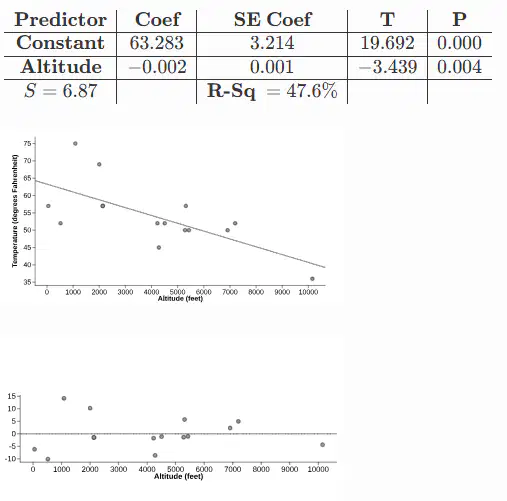
Interpret the value of r2 in context.
47.6% of the variation in the mean annual temperature is explained by the linear relationship with altitude.
6.87% of the variation in the mean annual temperature is explained by the linear relationship with altitude.
r^2 shows the direction of the relationship between variables.
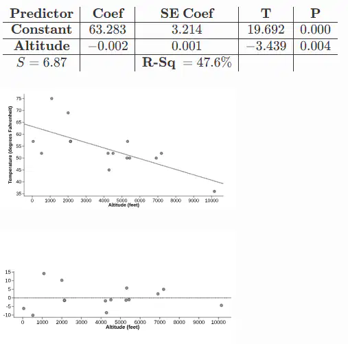
It would be reasonable to use the least squares regression line to predict the mean annual temperature for the peak of Mount Whitney, which has an altitude of 14,505 feet.
No, because 14,505 feet is likely outside the range of data used to create the regression line.
Yes, because regression lines can be used for any altitude.
Yes, as long as the altitude is above sea level.
No, because regression lines cannot be used for temperature predictions.
Match each description with the best possible correlation.
The temperature outside and ice cream sales
Positive Correlation
Total time spent playing video games and the number of cars you own
No Correlation
The number of days absent from school and your final grade in a class
Negative Correlation
Order the scatterplots from STRONGEST to WEAKEST correlation coefficients


Match the following correlation coefficients.
0.56
strong positive
-0.95
strong negative
0.48
weak positive
-0.25
weak negative
Drag the correct words into the blanks to interpret the r-value in context. Not all objects will be used.
The relationship between rain (inches) and plant height (inches) has an r-value of 0.34. Interpret the r-value in context.
There is a (a) (b) (c) relationship between (d) and (e)


What is the correlation for the following Scatter Plot.
Weak Positive
No Correlation
Strong Negative
Weak Negative
Strong Positive

What correlation coefficient best represents the scatter plot?
r=0.1
r=0.09
r=1
r=0.85