The population regression function provides the best (a)   to the CEF.

SIMPLE REGRESSION MODEL yi=β0+β1xi1+ui,i=1,…,N.(1)
The coefficient β1 measures the _____ in y associated with a unit _____ in x1, holding all of the unobservables constant.

(a)  

SIMPLE REGRESSION MODEL yi=β0+β1xi1+ui,i=1,…,N.(1)
If β0 and β1 solve the population least-squares problem their values ______ the expected value of the _____ difference between the dependent variable and the CEF.

(a)  

SIMPLE REGRESSION MODEL yi=β0+β1xi1+ui,i=1,…,N.(1)

The OLS estimator for β1 can be obtained by plugging in the _____ covariance between xi and yi and plugging in the _____ variance for xi.

(a)  

SIMPLE REGRESSION MODEL yi=β0+β1xi1+ui,i=1,…,N.(1)

If there were more than one x in (1), then the formula for β1 would be the _____, except xi1 would be replaced with the _____ from a regression of xi1 on the other xs.

(a)  

SIMPLE REGRESSION MODEL yi=β0+β1xi1+ui,i=1,…,N.(1)

The ______ theorem says you can control for other explanatory variables in estimating the effect of an x on y by either including the other variables directly or regressing y on the ______ from a regression of x on the other variables.

(a)  

SIMPLE REGRESSION MODEL yi=β0+β1xi1+ui,i=1,…,N.(1)

When the PRF includes more than one x, we say that β1 measures the (a)   effect of x1 (without necessary giving a causal interpretation).

SIMPLE REGRESSION MODEL yi=β0+β1xi1+ui,i=1,…,N.(1)

If E(ui|xi1)=0 in (1), xi1 is _____ of ui and the sampling error of β^1 equals ______ on average, which implies that β^1 is ______.

(a)  

SIMPLE REGRESSION MODEL yi=β0+β1xi1+ui,i=1,…,N.(1)

If E(ui|xi1)=0 in (1), the sampling error of β^1 converges to 0 and β^1 is (a)   .

REGRESSION MODEL WITH 2 EXPLANATORY VARIABLES: yi=β0+β1xi1+β2xi2+ui,,i=1,…,N,(2) where E(ui|xi1,xi2)=0.

If you omit xi2 from (2), β^1 will be biased ______ if β2 and cov(xi1,xi2) have the same ______.

(a)  

REGRESSION MODEL WITH 2 EXPLANATORY VARIABLES: yi=β0+β1xi1+β2xi2+ui,,i=1,…,N,(2) where E(ui|xi1,xi2)=0.
If yi1 is log wage, xi1 is education and xi2 is labor market experience, and you omit xi2 from (2), then β^1 will be biased ______ because β2 is _____ and cov(xi1,xi2) are _____ correlated.

(a)  

REGRESSION MODEL WITH 2 EXPLANATORY VARIABLES: yi=β0+β1xi1+β2xi2+ui,,i=1,…,N,(2) where E(ui|xi1,xi2)=0.

Let’s say you don’t omit xi2, but it is measured with error. Then β^2 will be (a)   . (unbiased/ biased down/ biased up)

REGRESSION MODEL WITH 2 EXPLANATORY VARIABLES: yi=β0+β1xi1+β2xi2+ui,,i=1,…,N,(2) where E(ui|xi1,xi2)=0.
R2 measures how much of the variance of the ______ variable is accounted for by the ______ variables.

(a)  

REGRESSION MODEL WITH 2 EXPLANATORY VARIABLES: yi=β0+β1xi1+β2xi2+ui,,i=1,…,N,(2) where E(ui|xi1,xi2)=0.
the test statistic for the null hypothesis that β2=1 is (a)   .

True or false. If corr(x,y)=0, y does not depend on x.

(a)  

True or false. If x causes y, the conditional distribution of y given x must depend on x.

(a)  

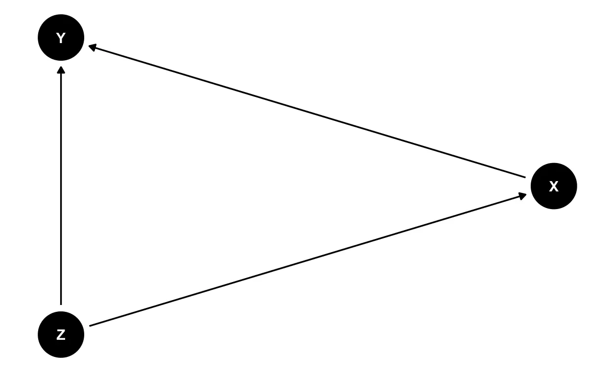
In the above DAG, Z is a (a)  

You can’t observe the effect of a treatment on an individual because you can’t observe their ______ outcome. In this sense, causal inference is fundamentally a ______ data problem.

(a)  

While individual treatment effects are not observable, you may be able to identify the average treatment effect (ATE), which is the difference in average (a)   outcomes.

Using the difference in sample average outcomes for treated and untreated individuals generally won’t work for estimating the ATE because potential outcomes (a)   (are/are not) independent of treatment assignment.

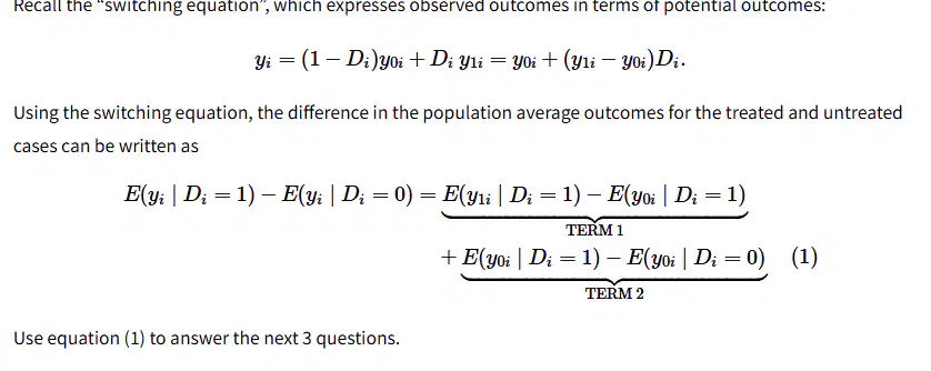
TERM 1 in (1) is

(a)  

TERM 1 in (1) is

(a)  

If treatment assignment is randomized, then TERM 2 equals ______ and TERM 1 equals the ______.

(a)  

If the potential outcomes are ______ of treatment assignment, the assignment mechanism is ______ and the difference in sample average outcomes for treated and untreated individuals will identify the ATE.

(a)  

Potential outcomes will be independent of treatment assignment if individuals are (a)   assigned to treated and untreated groups.

The conditional independence assumption (CIA) is a claim that there is a set of covariates that once you control for them, you can consider the potential outcomes to be ______ of treatment assignment. The CIA is a claim of ______ and is untestable.

(a)  

To estimate the ATE under a CIA, you also need overlap, which is the ability to observe ______ and ______ units for any set of covariate values.

(a)  

If you have a set of control variables for which a CIA holds, you can identify the average effect of the treatment on the outcome by running a regression of the outcome on the (a)   from a regression of the treatment dummy on the controls.

The standard 2×2 DD analysis compares the difference in average outcomes for the _____ observations before and _____ treatment with the difference in mean outcomes for the control observations _____ and _____ treatment.

(a)  

A DD analysis targets the average treatment effect on the (a)   .

The target estimand cannot be estimated directly because E(y0|g=1,t=1) is (a)   .

The key identifying assumption in a DD analysis is that the treated and untreated outcomes would follow _____ trends in the _____ of the treatment.

(a)  

A simple before vs after comparison of treated observations misses the (a)   in the outcome not associated with treatment.

A simple comparison of treated vs control observations after treatment misses factors that cause non-random (a)   into treatment.

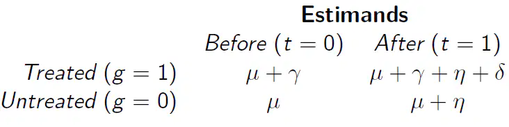
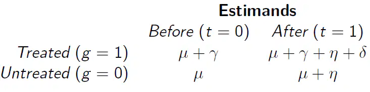
The parameter γ reflects the average difference between _____ and _____ outcomes before treatment.

(a)  

The parameter η reflects the average difference in outcomes _____ and _____ treatment for the untreated group.

(a)  

The parameter η also reflects the _____ average difference in outcomes between periods 0 and 1 for the _____ group.

(a)  

If η varied by group, the (a)   assumption would not hold.

The parameter δ represents the (a)   .

The standard 2×2 DD analysis can be carried out by regressing the outcome on a _____ dummy, a period _____, and their _____.

(a)  

y=μ+γtreat+ηafter+δtreat⋅after+u

(a)  

A regression formulation of a DD design is appealing because it

- facilitates standard error estimation

- generalizes for multiple time periods and treatment groups

- accommodates (a)  

We described a TWFE model as a regression model for data with both a (a)   and time dimension.

Estimating a TWFE model with data on multiple groups and variation in treatment timing can identify the ATT if the treatment effect is (a)   .

Computing the correct standard errors for TWFE estimates usually requires _____ at the group level to account for _____ and _____ correlation.

(a)  

Regression provides the best (a)   approximation to the
conditional expectation function

this means that population regression coefficients minimize the
(a)   between the outcome and the approximation.

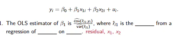
(a)  

yi = β0 + β1x1i + β2x2i + ui .
1. If x2 was omitted from the regression, ˆβ1 would be biased unless β2 =
_____ or x1 and x2 were _____.

(a)  

yi = β0 + β1x1i + β2x2i + ui .
the test statistic for the null that β1 = 0 is (a)   .

The results in Project Table 5 show that omitting Education caused
the estimated Female coefficient to be biased _____. The direction
of the bias follows facts that Education is _____ correlated with
Female and _____ correlated with log wages.

(a)  

Controlling for education causes the estimated gender wage gap to
_____ by about _____ percentage points.

(a)  

What sort of standard errors should you always report?

(a)  

The metric that we use to compare prediction models is (a)   or MSPE.

consider two estimators of the population mean μ, μ^ and μ~. Assume that μ^ has a N(0,1) sampling distribution, μ~ has a N(.5,(.5)2) sampling distribution, and the true mean of the population is 0.

Mean squared error of (μ^)= (a)   .

consider two estimators of the population mean μ, μ^ and μ~. Assume that μ^ has a N(0,1) sampling distribution, μ~ has a N(.5,(.5)2) sampling distribution, and the true mean of the population is 0.

Mean squared error of (μ~)= (a)   .

consider two estimators of the population mean μ, μ^ and μ~. Assume that μ^ has a N(0,1) sampling distribution, μ~ has a N(.5,(.5)2) sampling distribution, and the true mean of the population is 0.

E(μ^)−μ= _____, which implies μ^ is _____.

(a)  

consider two estimators of the population mean μ, μ^ and μ~. Assume that μ^ has a N(0,1) sampling distribution, μ~ has a N(.5,(.5)2) sampling distribution, and the true mean of the population is 0.

Although μ~ is (a)   , it has a lower mean squared error.

consider two estimators of the population mean μ, μ^ and μ~. Assume that μ^ has a N(0,1) sampling distribution, μ~ has a N(.5,(.5)2) sampling distribution, and the true mean of the population is 0.
R¯2 penalizes the inclusion of an additional explanatory variable if its associated t-statistic is less than (a)   .

Machine learning that involves predicting an outcome with a set of explanatory variables is called (a)   learning.

Choosing the best-performing ML model involves empirically tuning model complexity through (a)   .

Cross-validation begins by dividing the data into _____ and _____ samples.

(a)  

The training sample is divided into folds, one of which is held out for _____ while the others are used to _____ the model.

(a)  

Cross-validation involves computing the _____ for each fold and _____ them over all folds.

(a)  

Cross-validation is repeated for different values of λ, which determines the strength of the (a)   imposed by the regularizer.

LASSO is a shrinkage estimator that also performs variable _____ by forcing the coefficients of the least relevant variables to be equal to _____.

(a)  

Larger ______ statistics and smaller ______ values indicate stronger evidence ______ (for/against) the null hypothesis.

(a)  

The test statistic for whether a explanatory variable has a statistically significant association with the dependent variable is the ratio of the explanatory variable’s coefficient ______ to its _____.

(a)  

The R function lm gives the wrong standard errors, test statistics and confidence intervals because it ignores (a)   .

The modern approach means we should always report (a)   standard errors and test statistics.

The modern approach to regression inference allows for the variance of the errors to depend on the (a)   variables.

Basic OLS inference is grounded in the application of the CLT, which says that the ______ distribution of the OLS estimator can be regarded as approximately _____ for large samples.

(a)  

True or false: R2 is centrally important for doing causal inference.

(a)  

Unlike in standard regression analysis, in RD designs there is no (a)   in treated and control units because individuals with different values of D, the treatment, have different values of the covariate by construction.

In a sharp RD design, the conditional _________ assumption holds automatically because treatment assignment is determined solely by the cutoff value of the _______ variable.

(a)  

In a fuzzy RD design, the cutoff value of the running variable determines the (a)   of treatment.

The key identifying assumption of an RD design is that the average _____ outcomes are _____ through the cutoff.

(a)  

Under the assumptions of a sharp RD design, you identify an

(a)  

The blue and red lines are linear regression approximations to the CEFs for the (a)   outcomes.

the regression specification that is consistent with the blue and red lines is Outcomei=β0+δAboveCutoff i+β1RunningVariablei+β2(AboveCutoff i×RunningVariablei) + ui

true/false

(a)  

Under the key identifying assumption of a sharp RD design, the model in Question 7 identifies

δ=E(y1i−y0i|RunningVariablei=50)

true/false

(a)  

The basis for an RD analysis should be apparent in a binned ______ plot of the outcome and the _____ variable.

(a)  

In general, the RD specification should include a low-order _____ in the running variable and an interaction of the running variable with the _____ indicator.

(a)  

The distribution of the running variable should show

(a)  

An RD analysis of baseline covariates should show no evidence of (a)   among them.

Including the baseline _____ in the regression model (should/should not) _____ affect the estimated treatment effect.

(a)  

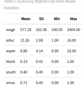
The average wage of the young men in Card’s sample is $ ______ and the standard deviation of wages is $ ______. (Round to the nearest cent.)

(a)  

Approximately ______ percent of the sample lives in the South and ______ lives in a city.

(a)  

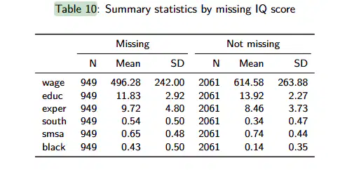
On average, men with complete IQ test score data earn approximately $______ more per hour (round to the nearest dime) and have _____ more years of schooling (round to the nearest year).

(a)  

On average, men with missing IQ test scores are ______ points _____ (more/less) likely to be from the south and _____ points _____ (more/less) likely to live in a city.

(a)  

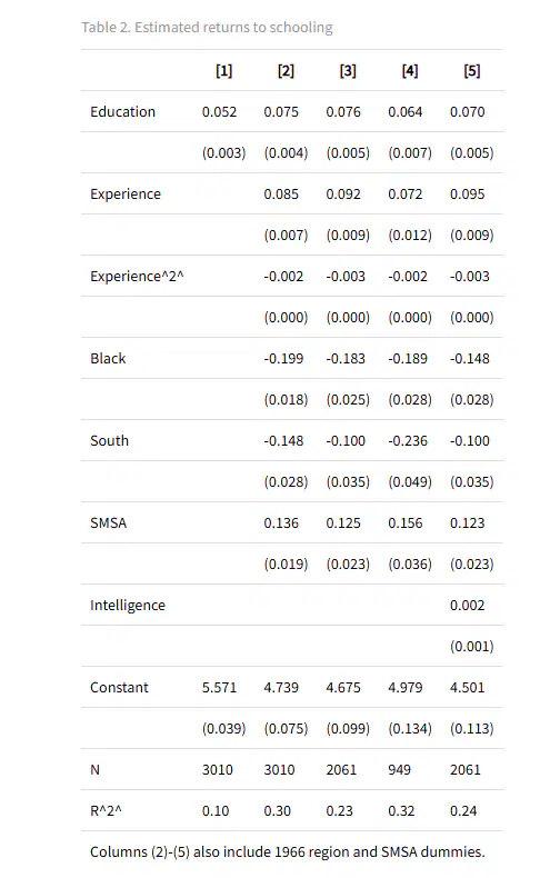
The simple regression of log wages on years of education yields an estimated coefficient of ______ (report 3 decimal places), which suggests an additional year of schooling is associated with a ______ % (report one decimal place) increase in wages. This result ______ (is/ is not) statistically significant at the 5% level.

(a)  

Adding the control variables in Column [2] increases the estimated return to schooling by (a)   percentage points (report one decimal place).

The results in Column [2] indicate living in a city is associated with a statistically ______ average wage premium of ______ % (report one decimal place).

(a)  

Based on the results in Column [2], the estimated return to the first year of experience is about (a)   % (report one decimal place). ([0.085-(2)(0.002)(1)] x 100 =

Including the IQ test score as an ability proxy decreases the estimated return to schooling by about (a)   percentage points (report one decimal place).

The result reported in Column [5] is expected because the test score has a ______ effect on wages and is ______ correlated with education.

(a)  

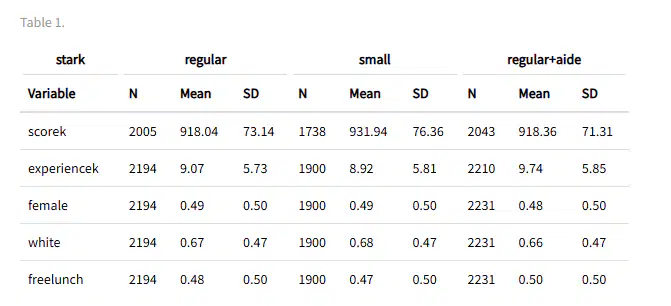
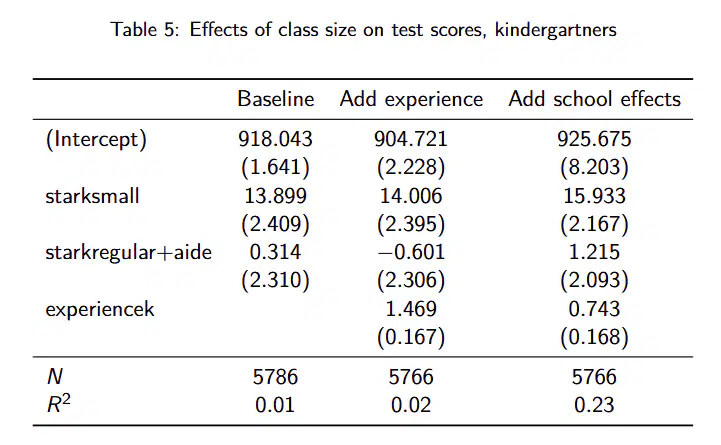
The difference between small and regular-class mean scores for kindergarteners is about (a)   points (report one decimal place).

Under _____ assignment of students to class type, the difference between small and regular class mean scores can be regarded as the _____ of small class size on test scores.

(a)  

the difference between small and regular class mean scores, is it meaningful? One way to measure the magnitude of this effect is to compare the effect size to the size of a standard deviation in the baseline. This difference amounts to about (a)   of a standard deviation in the baseline regular-class sample. (Give a fraction or percent approximation).

Average teacher experience ranges between _____ and _____ years across class type (round to one decimal)..

(a)  

The average percentage of free-lunch students in each class type is between _____ and _____ percent.

(a)  

Based on the information in Table 1, Project STAR had good _____ and covariate _____ across class types.

(a)  

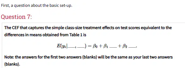
(a)  

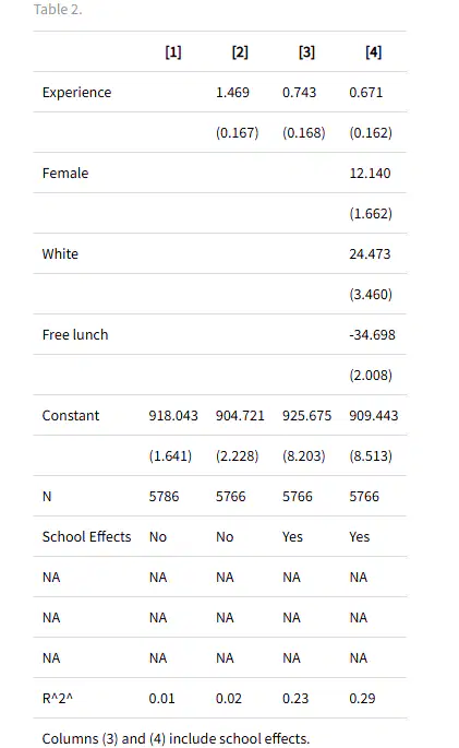
The estimated small-class effect in Column (1) is (a)   to the difference in means calculated from Table 1.

The result in Column (1) is statistically significant at the (a)   -percent level.

The results in Column (1) indicate that the effect of adding an aide to a regular class is just under 1/3 of a point and statistically (significant/insignificant) (a)   .

The t statistic for the teacher-experience coefficient estimate in Column (2) is (a)   . (Round to one decimal).

Adding the gender, race and free-lunch controls improves the overall fit of the regression by _____ percentage points (round to one decimal), but has _____ impact on the estimated small-class effect reported in Column (3).

(a)  

Overall, the simple differences-in-means result _____ (is/is not) highly robust, holding up even when you _____ for a range of student and school characteristics.

(a)  

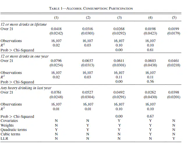
CD in the Results subsection titled ‘‘A. Alcohol Consumption’’ show that drinking increases after the 21st birthday on both the

(a)  

In Table 1. Alcohol Consumption: Participation, their preferred specification indicates a statistically significant (a)   percentage-point effect on the likelihood of having 12 or more drinks in a year. (Answer with an integer value).

This 6 percentage-point effect translates into about a/an (a)   percent increase on the likelihood of having 12 or more drinks in a year. (Answer with an integer value, and refer to relevant text within Result subsection A).

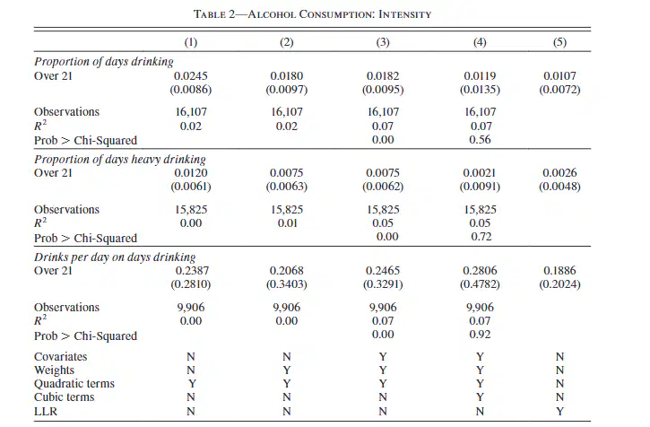
In Table 2. Alcohol Consumption: Intensity, their preferred specification indicates a (a)   percentage-point increase in the proportion of days drinking. (Answer with an integer value, and refer to relevant text within Result subsection A).

This percentage-point effect translates into about a/an (a)   percent increase in the proportion of days drinking. (Answer with an integer value.)

CD lump all causes potentially related to _____ into the external category and all causes unrelated to ______ into the _______ (internal/external) category.

(a)  

The distinction between causes of death is important because estimating the treatment effect on (a)   causes should function as a falsification exercise.

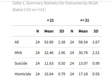
Deaths from motor vehicle accidents for under 21-year-olds comprise about (a)   percent of all deaths.(Round to the nearest integer.)

The homicide rate for under 21-year-olds is about _____ per _____. (You may need to refer to the paper here, and round to the nearest integer.)

(a)  

Overall, MVA deaths (increase/decrease/stay the same) (a)   after age 21.

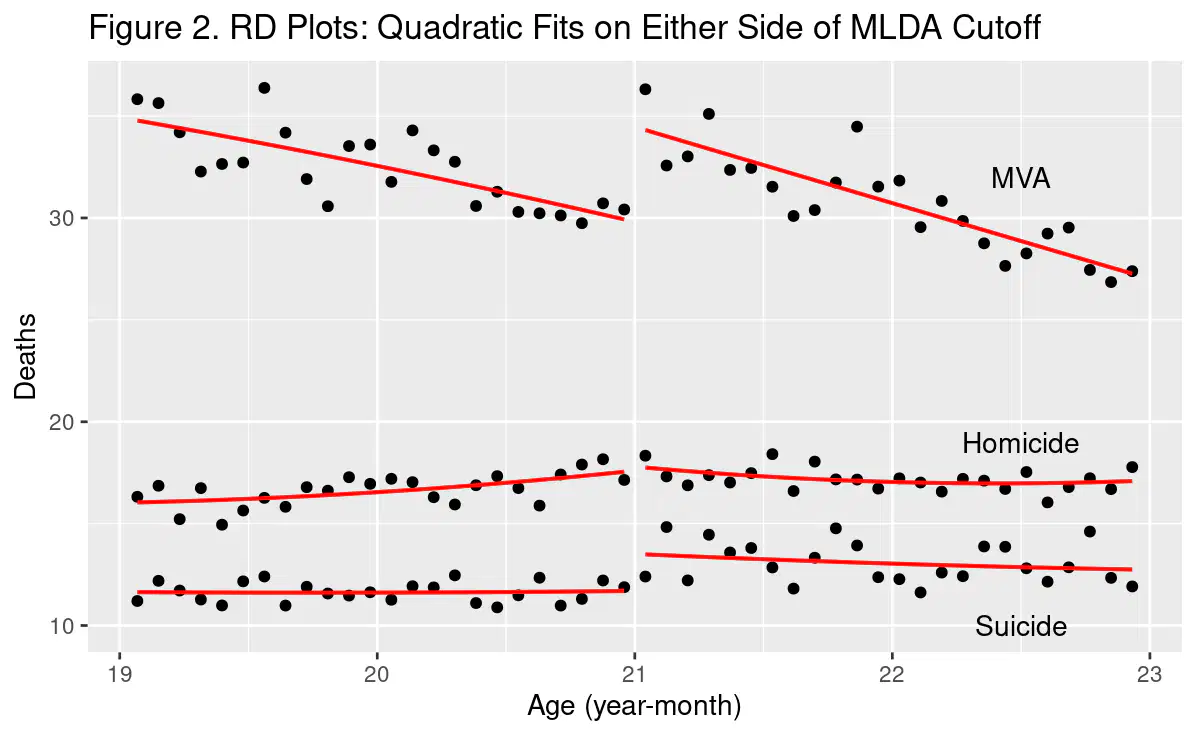
Just after age 21, MVA deaths appear to rise by almost (a)   per 100,000. (Round to the nearest integer.)

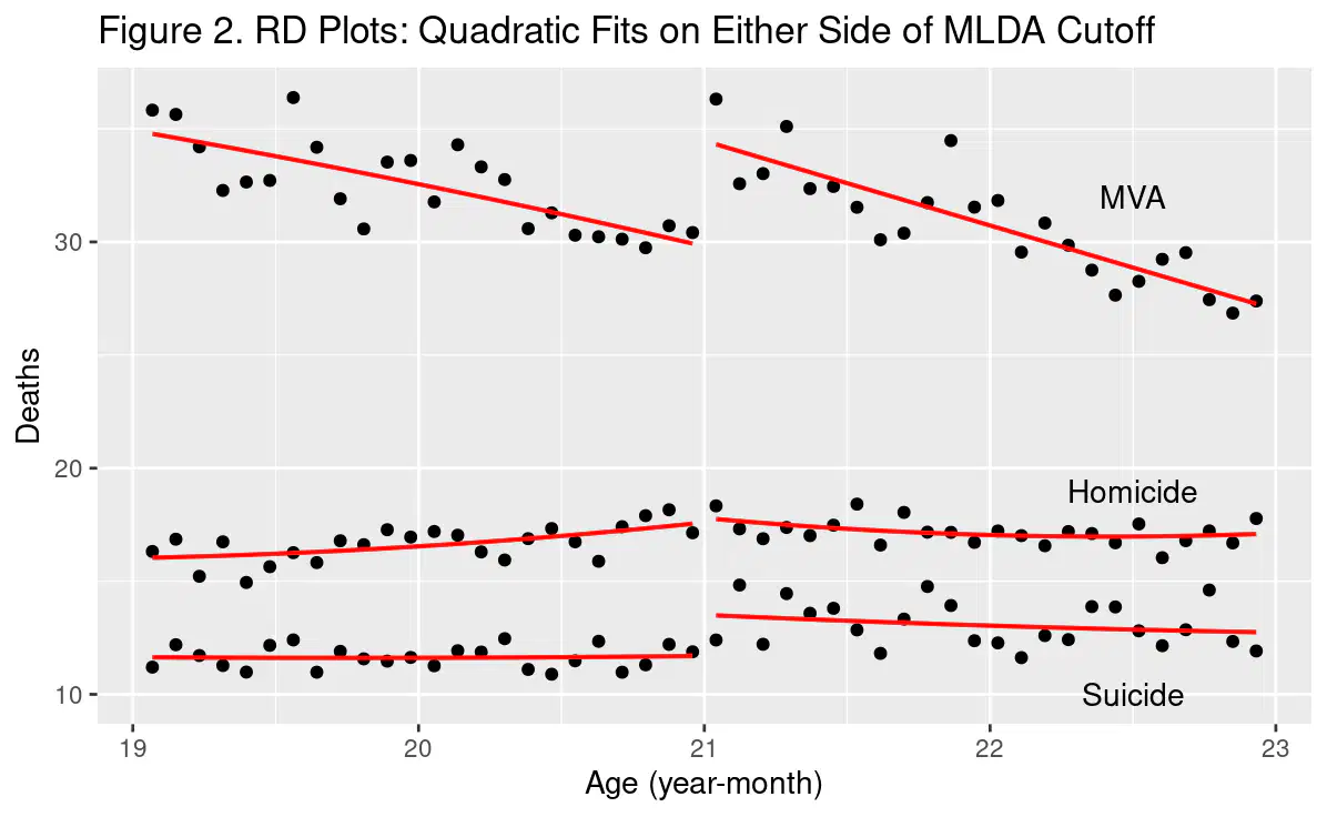
Just after age 21, suicides appear to rise by about (a)   per 100,000. (Round to the nearest integer.

The homicide rate (does/does not) (a)   change at age 21.

The results in Table 2 suggest that MVA deaths increased from _____ to _____ (round to two decimals for both blanks) at age 21, depending on the whether we use a simple _____ (linear/quadratic/polynomial) or flexible _____ (linear/quadratic/polynomial) specification.

(a)  

The estimated effects on MVA deaths (a)   (are/are not) statistically significant at the 5% level.

The MVA effect reported in Column (2) and the baseline MVA death rate of 32.5 suggests an increase in MVA deaths of _____ percent (report 1 decimal place), which (is/is not) _____ consistent with CD’s MVA findings.

(a)  

The results in Table 2 suggest that suicides increased from _____ to _____ (round to two decimals) at age 21, depending on the whether we use a simple _____ (linear/quadratic/polynomial) or flexible _____ (linear/quadratic/polynomial) specification.

(a)  

The estimated effects of turning 21 on suicides (are/are not) (a)   statistically significant at the 5% level.

The results in Table 2 indicate a very _____ and statistically _____ effect of turning 21 on homicides.

(a)  

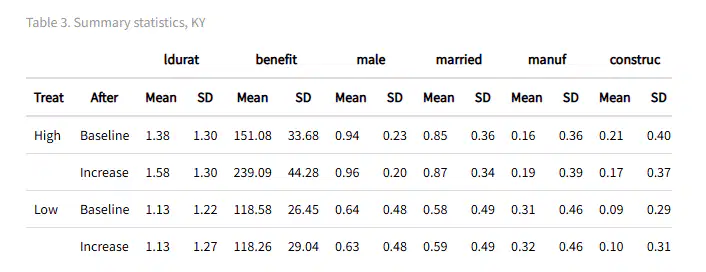
The ldurat difference in differences is (a)   .

The benefit difference in differences is (a)   .

The high-earner group is (more/less) _____ male and (more/less) _____ married, but the male and married shares (do/do not) _____ change over time for either group.

(a)  

The high-earner group is (more/less) _____ likely to work in maufacturing and (more/less) _____ likely to work in construction, and the share of high earners in contruction (rises/falls) _____ by _____ points after the WBA increase.

(a)  

Based on Table 1, average time out of work rose (a)   % because of the WBA increase.

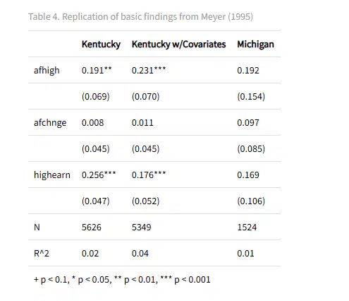
Column (1) indicates that time out of work (did/did not) (a)   rise for low earners.

Column (1) indicates that average time out of work was _____ % (higher/lower) _____ for high earners. (Report to one decimal place.)

(a)  

The results in column (1) suggest that time out of work rose (a)   % in Kentucky because of the WBA increase. (Report to one decimal place.)

The standard error for the estimated DD coefficient is _____ , which implies that the result is significant at the _____ % level.

(a)  

Controlling for gender, industry affiliation and injury type (increases/decreases) _____ the DD coefficient estimate for KY by _____ percentage points .

(a)  

Controlling for gender, industry affiliation and injury type (increases/decreases) _____ the overall fit of the regression by _____ percentage points.

(a)  

Still, the overall fit reported in Column (2) is too low for the regression results to be trustworthy.

(a)  

The results in column (3) suggest that time out of work rose (a)   % in Michigan because of the WBA increase. (Report to one decimal place.)

The t statistic for the estimated DD coefficient in Column (3) is _____ (round to two decimal places), which implies you (can/cannot) _____ reject the null at the 5% level.

(a)  

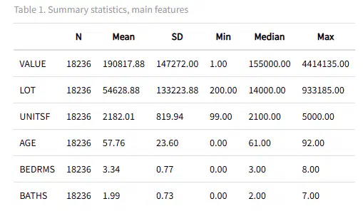
The average house value in the sample is $ (a)   . (Round to the nearest dollar.)

The median house value in the sample is $ (a)   . (Round to the nearest dollar.)

The average house in the sample is (a)   square feet. (Round to the nearest integer.)

The largest house in the sample is (a)   square feet. (Round to the nearest integer.)

The coefficient plot shows how the estimated coefficients vary with the λ values and which variables are (a)   as λ is increased.

The CV(M) plot shows how (a)   varies with λ.

[1] "Lasso min CV(M) estimate: 0.474418419590542"

[1] "Lasso CV(M)-minimizing lambda value: 0.00233733145841437"

[1] "Number of nonzero lasso coefficients at optimal lambda: 52 out of 85"

The CV(M) is minimized using a λ value of _____ and the minimized value of CV(M) is _____. (Report to 3 decimal places.) Using the optimal λ, lasso retains _____ explanatory variables.

(a)  

[1] "Lasso MSPE: 0.542950794357761"

[1] "OLS MSPE: 0.543935140494568"

The test-sample MSPEs are _____ for lasso and _____ for OLS. (Round to 3 decimal places and in X.XXX format.)

(a)  

[1] "Lasso MSPE: 0.542950794357761"

[1] "OLS MSPE: 0.543935140494568"

The lasso improvement over OLS is about (a)   percent. (Round to the nearest tenth of a percent).

Write down the regression model that corresponds to the following

code: lm(y~x1, data).

(a)  

2. The first (reading from the left) vertical dotted line indicates the

Lasso specification that minimizes the _____ in the cross-_____

process of training.

(a)  

3. The LPM results in Table 5 suggest that another year of education

increases the likelihood of being in the labor force by (a)