
NEW
Font size
S
M
L
XL
 Worksheets
Chapter 5 excel
Total questions: 50
Worksheet time: 13hrs 30mins
Name
Class
Date
1.
In Microsoft Excel, the way to hide a Sheet in Excel is:
a)
A. Select the Sheet needed by clicking the select button → Hide
b)
B. Select the Sheet needed by pressing Ctrl + A → Right-click → Hide
c)
C. Right-click on the name of the Sheet needed → Hide
d)
D. Left-click on the name of the Sheet needed → Hide
2.
In Microsoft Excel, the way to open an additional new Sheet in a file is:
a)
A. Right-click on any Sheet in the file → Insert → Worksheet → OK
b)
B. Right-click on any Sheet in the file → Insert → MS Excel → OK
c)
C. Left-click on any Sheet in the file → Insert → MS Excel → OK
d)
D. All of the above options are false
3.
In Microsoft Excel, the symbol ### in a spreadsheet column indicates:
a)
A. Data in the column has an error
b)
B. Data format in the column has an error
c)
C. Calculation result has an error
d)
D. Column width is insufficient to display numerical data
4.
In Microsoft Excel, the symbol #VALUE in a spreadsheet indicates:
a)
A. Column width is insufficient to display numerical data
b)
B. Data used for calculation has an error
c)
C. No result
d)
D. Function input is incorrect
5.
In Microsoft Excel, the symbol #NAME... in a spreadsheet indicates:
a)
A. Incorrect function name input
b)
B. Incorrect data input
c)
C. Row height is insufficient to display data
d)
D. Incorrect data input and row height is insufficient to display data
6.
In Microsoft Excel, the key combination that immediately moves the cursor to the first cell (A1) is:
a)
A. Ctrl + Shift + Home
b)
B. Ctrl + Shift + Page Up
c)
C. Shift + Home
d)
D. Ctrl + Home
7.
In Microsoft Excel, cell A1 has the value Nguyễn Lan, cell B1 has the value Anh. In cell C1, the formula entered is = A1 + B1; the result is:
a)
A. Nguyễn Lan Anh
b)
B. Nguyễn LanAnh
c)
C. #VALUE
d)
D. No result
8.
In Microsoft Excel, cell A1 has the value 9.78 (right-aligned data). In cell B1, the formula entered is = Int(A1); the result is:
a)
A. 9.5
b)
B. #VALUE
c)
C. 10
d)
D. 9
9.
In Microsoft Excel, cell A1 has the value 9.78 (left-aligned data). In cell B1, the formula entered is = Int(A1); the result is:
a)
A. 9.5
b)
B. #VALUE
c)
C. 10
d)
D. 9
10.
In Microsoft Excel, cell A1 has the value 13/01/2020 (left-aligned data). In cell B1, the formula entered is = day(A1); the result is:
a)
A. #VALUE
b)
B. 13
c)
C. 01
d)
D. 2020
11.
In Microsoft Excel, cell A1 has the value 13/01/2020 (right-aligned data). In cell B1, the formula entered is = month(A1); the result is:
a)
A. #VALUE
b)
B. 1
c)
C. 13
d)
D. 2020
12.
In Microsoft Excel, cell A1 has the value 13/01/2020 (right-aligned data). In cell B1, the formula entered is = year(A1); the result is:
a)
A. #VALUE
b)
B. 20
c)
C. 1920
d)
D. 2020
13.
In Microsoft Excel, cell A1 has the value 20, cell B1 has the value 7. In cell C1, the formula that results in 6 is:
a)
A. = mod(A1; B1)
b)
B. = mod(A1/B1)
c)
C. = mod(B1;A1)
d)
D. = mod(B1/A1)
14.
In Microsoft Excel, column A from cell A2 to A10 contains numerical data representing the IT exam scores. In cell B2, enter the formula to rank students by score from highest to lowest (Highest rank is 1). Which formula is correctly entered:
a)
A. = rank(A2;AS2:A10;1)
b)
B. = rank(A2;A2:A10;0)
c)
C. = rank(A2;A2:A10;1)
d)
D. = rank(A2:A2:A10;:0)
15.
In Microsoft Excel, cell A1 has the value 0, cell B1 has the value 7. In cell C1, the formula entered is = B1/A1, the result is:
a)
A. ERROR
b)
B. DIV/0
c)
C. #DIV/0
d)
D. #VALUE
16.
In Microsoft Excel, the operator used when comparing for "not equal to" is:
a)
A. &
b)
B. #
c)
C. ><
d)
D. <>
17.
In Microsoft Excel, the operator used for concatenating strings (text strings) is:
a)
A. &
b)
B. and
c)
C. link
d)
D. +
18.
In Microsoft Excel, in cell A1, the formula entered is = and(5>4;9<5) the result is:
a)
A. TRUE
b)
B. Đúng (Correct)
c)
C. Sai (Incorrect/False)
d)
D. FALSE
19.
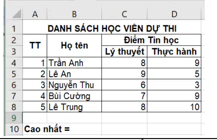
In Microsoft Excel, given the data above [related to columns C and D], in cell C10 enter the formula: = max(C4:D8); the result is:
a)
A. 8
b)
B. 9
c)
C. 10
d)
D. 7
20.
In Microsoft Excel, in cell A1, the formula entered is = or(10>4;20<=5) the result is:
a)
A. Đúng (Correct)
b)
B. TRUE
c)
C. Sai (Incorrect/False)
d)
D. FALSE
21.
In Microsoft Excel, in cell A1, the formula entered is =ROUND(15/2; -1), which of the following results is correct:
a)
A. 7
b)
B. 0
c)
C. 10
d)
D. None of the results
22.
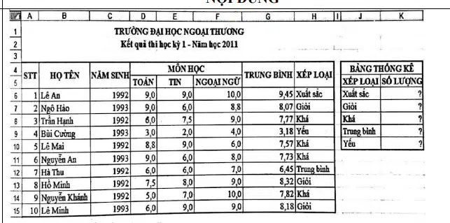
According to the illustration, to find the total number of students classified as Excellent, Good, Fair, Average, Poor; which formula should be placed in cell K6:
a)
A. = COUNT(G6:G15;J6)
b)
B. = COUNT(&G6:G$15;J6)
c)
C. = COUNTIF(H6:H15;J6)
d)
D. = COUNTIF(G6:G15;16)
23.
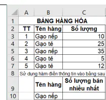
In MS Excel, given the data above [related to DMAX], to calculate the maximum Quantity sold for Rice, in cell C10 enter the formula:
a)
A. =DMAX(A2:C7;3;B9:B10)
b)
B. =DMAX(A3:C7;3;B9:B10)
c)
C. =DMAX(A3:C7;3;B10)
d)
D. =DMAX(A2:C7;3;B10)
24.
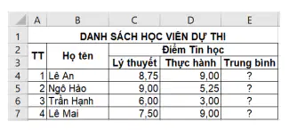
In Microsoft Excel, given the data above, to calculate the average value, in cell E4 use the formula: =INT(ROUND((C4+D4);0))/2; the result in cell E4 is:
a)
A. 8
b)
B. 9
c)
C. 8.5
d)
D. 8.25
25.
In Microsoft Excel, cell A1 has the value Thành phố Hà Nội. In cell B1, the formula entered is = Left(A1;3) the result is:
a)
A. Thà
b)
B. Th and the grave accent ()**
c)
C. Tha
d)
D. Nội
26.
In Microsoft Excel, cell A1 has the value Thành phố Hà Nội. In cell B1, the formula entered is = Right(A1;3) the result is:
a)
A. Nôi
b)
B. Nội
c)
C. Tha
d)
D. Thà
27.
In Microsoft Excel, to edit data or a formula in a cell without re-entering it, perform:
a)
A. Click the mouse on the cell to be edited and press F4
b)
B. Click the mouse on the cell to be edited and press F3
c)
C. Click the mouse on the cell to be edited and press F5
d)
D. Double-click the mouse on the cell to be edited
28.
In Microsoft Excel, what type of addresses are the following: A1,B5, C6, $L9, D7
a)
A. Relative addresses
b)
B. Absolute addresses
c)
C. Mixed addresses
d)
D. Includes all three types of addresses above
29.
In Microsoft Excel, the way to sort a payroll list (without merged cells) in ascending order based on the "Total income" of staff in the agency, after highlighting the payroll table, is:
a)
A. Go to Data → Sort → Sort by: Select the "Total income" column → Select Descending → OK
b)
B. Go to Table → Sort → Sort by: Select the "Total income" column → Select Ascending → OK
c)
C. Select the "Payroll" table → Go to Table → Sort → Sort by: Select the "Total income" column → Select Ascending → OK
d)
D. Select the "Payroll" table → Go to Data → Sort → Sort by: Select the "Total income" column → Select Ascending → OK
30.
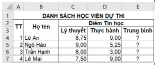
In Microsoft Excel, given the data above, to calculate the average value = (Theory + Practice)/2, in cell E4 use the formula:
a)
A. =average(C4:C8)
b)
B. =average(C4:D4)
c)
C. =average(C4:$DS4)
d)
D. =average(C4:D4)
31.
In Microsoft Excel, suppose the system date is 01/01/2020. In cell A1, the formula entered is = year(today()) - 1990 the result is:
a)
A. 30
b)
B. #VALUE
c)
C. #NAME...
d)
D. 31
32.
In Microsoft Excel, before using the Subtotals command:
a)
A. Data rearrangement is not necessary
b)
B. Data must be copied to another range and rearrangement is not necessary
c)
C. Data must be rearranged (Sort)
d)
D. Data must be filtered to another range and rearrangement is not necessary
33.
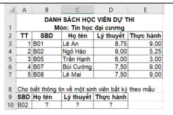
In Microsoft Excel, given the data above [related to DGET function], in cell B10 enter the formula:
a)
A. =DGET(A3:E7;3;A9:A10)
b)
B. =DGET(SAS2:E7;2;A10)
c)
C. =DGET(A2:E7;3;A9:A10)
d)
D. =DGET(A3:E7;3;A10)
34.
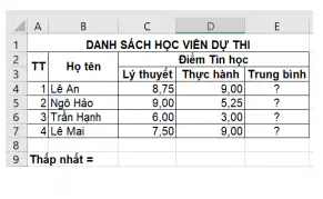
In Microsoft Excel, given the data above [related to min function], in cell C10 enter the formula: = min(C4:D8); the result is:
a)
A. 6
b)
B. 5.25
c)
C. 3
d)
D. 5
35.
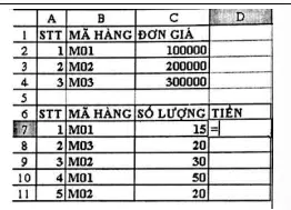
In Microsoft Excel, given the table [related to VLOOKUP]: To calculate Amount = Quantity * Unit Price, in cell D7 enter the formula:
a)
A. =C7 * vlookup(B7;A1:C4;3;0)
b)
B. =C7 * vlookup(B7;A1:C4;3;0)
c)
C. =C7 * vlookup (B7;A1:C4;3;0)
d)
D. =C7 * vlookup(B7;B1:C4;2;0)
36.
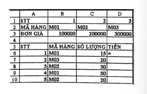
In Microsoft Excel, given the table [related to HLOOKUP]: To calculate Amount = Quantity * Unit Price, in cell D6 enter the formula:
a)
A. = C6 * Hlookup(B6; A1:D3;3;0)
b)
B. = C6 * Hlookup(B6;A1:D33;3;0)
c)
C. = C6 * Hlookup(B6; A2: D3;2;0)
d)
D. = C6 * Hlookup(B6;A1:D3;3;0)
37.
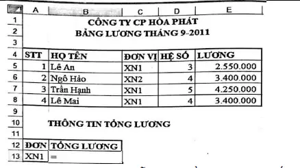
Given the payroll table [related to SUMIF]. Required calculation: Find the Total salary of any unit. In cell B13, use the formula:
a)
A. =sumif(C4:CS8,C5,SES5:E$8)
b)
B. =sumif(C4:E8;A11:A13;E4:E$8)
c)
C. =sumif(CS4:C$8;A11:A13;E5:E8)
d)
D. =sumif(C4:C8;A13;E4:E8)
38.
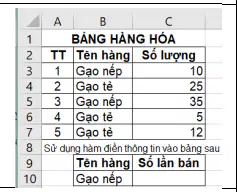
In MS Excel, given the data above [related to DCOUNT], to calculate the number of times sticky rice was sold, in cell C10 enter the formula:
a)
A. =DCOUNT(A2:C7;3;B9:B10)
b)
B. =DCOUNT(A2:C7;2;B9:B10)
c)
C. =DCOUNT(A3:C7;3;B9:B10)
39.
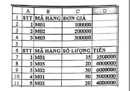
In Microsoft Excel, given the table. To summarize (Subtotals) the quantity and amount collected for each item, the key field used is:
a)
A. Item Code (Mã hàng)
b)
B. Quantity and Amount
c)
C. Quantity
d)
D. Amount
40.
In Microsoft Excel, given the table. To summarize (Subtotals) the quantity and amount collected for each item, the following columns must be copied to another range:
a)
A. Item Code and Amount
b)
B. Quantity and Amount
c)
C. Item Code and Quantity
d)
D. Item Code, Quantity and Amount
41.
After entering an Excel formula and pressing Enter, the cell may display error messages such as #REF!, #VALUE!, #N/A. These error messages mean, respectively:
a)
A. Function name not found, invalid reference, reference value does not exist
b)
B. Invalid reference, wrong data type, data not found
c)
C. Reference value does not exist, function name not found, invalid reference
d)
D. The set used for calculation is empty
42.
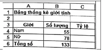
In the figure on the side, to calculate the percentage, the formula that should be used is:
a)
A. =B4/B6
b)
B. =BS4/B6
c)
C. =B4/B6
d)
D. =B4/SB$6
43.
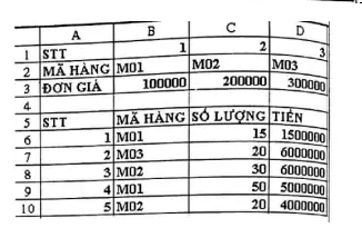
Suppose cell A1102 has the data BM00900F. In cell B1102 and cell C1102, the formulas entered are respectively: = VALUE(MID(A1102;3;5)) and = MID(A1102:3;5) the results are:
*note: Cảm giác cái hình không giống cái đề lắm :))
a)
A. 900 and 00900
b)
B. 00900 and 00900
c)
C. 0900 and 900
d)
D. All a, b, c are false
44.
The formula in cell F63 is: = C2+H2. When copied to cell H66, it will be in the form:
a)
A. =C3+I2
b)
B. =CS+J2
c)
C. =DI+I2
d)
D. =C2+I3
45.
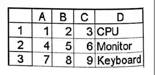
Given the spreadsheet as shown. The results of the three formulas: =COUNT(A1:D3), =COUNTIF(A1:D3; "<5"), =SUMIF(A1:A3; "<5"; C1:C3) are, respectively:
a)
A. 9, 4, 9
b)
B. 5, 9, 9
c)
C. 9, 5, 7
d)
D. 9, 9, 7
46.
The following statements are true in Excel: I. AutoFilter feature allows filtering records that satisfy conditions to another location only within the current sheet. II. AutoFilter feature cannot filter using the "and" style between conditions. III. Subtotal feature is used not only to calculate subtotals for data ranges. IV. Subtotal feature always creates a Grand Total row below the last Subtotal row.
a)
A. All 4 statements are correct
b)
B. Statement III is incorrect
c)
C. Statements II and IV are incorrect
d)
D. Statements I, II and IV are incorrect
47.
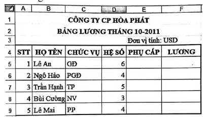
Given the database range as shown: To perform the calculation: Allowance = 150 USD if the position is "GĐ" (Director), 100 USD if the position is "TP" (Department Head) or PGĐ (Deputy Director), 50 USD for all other cases. In cell E5, the formula to be entered is:
a)
A. =IF(C5=“GĐ”;l50;IF(OR(C5=“TP”;C5=“PGĐ");100;50))
b)
B. =IF(C5=“GĐ”;150;IF(C5=“TP”;100; IF(B5“PGĐ”,100;50)))
c)
C. =IF(C5=”GĐ”;150;IF((C5=“TP”) OR (B5=“PGĐ”);100;50))
d)
D. =IF(C5=“GĐ”;150; IF(AND(C5=“TP”;B5="PGĐ`);100;50))
48.
Which of the following statements about Excel is incorrect:
a)
A. The width of multiple columns cannot be changed simultaneously
b)
B. The width of multiple columns can be changed simultaneously
c)
C. A command can be used to change the width of columns to fit the data
d)
D. Multiple lines of text can be written in one Cell
49.
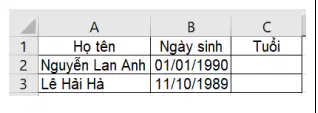
In the screen shown, to calculate the age in cell C2, use the formula:
a)
A. =year(today)-B2
b)
B. =year(today())-year(B2)
c)
C. =year(today())-B2
d)
D. =year(today)-year(B2)
50.
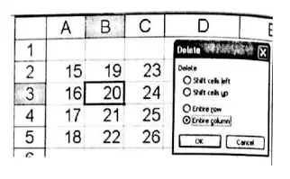
In the figure on the side, perform the operation: Right-click on cell B3 → Select Delete → Select Entire column. After pressing "OK", cell B3 will contain the value:
a)
A. 16
b)
B. 19
c)
C. 21
d)
D. 24
Reset