4 Key Questions to Understanding Aggregate Supply

Here we are going to explore everything you need to know about both short-run and long-run aggregate supply. Both of these supply curves are important components to the aggregate supply/aggregate demand model (AS/AD) and the AS/AD model is essential to understanding the macroeconomy.

1. What is short-run aggregates supply?

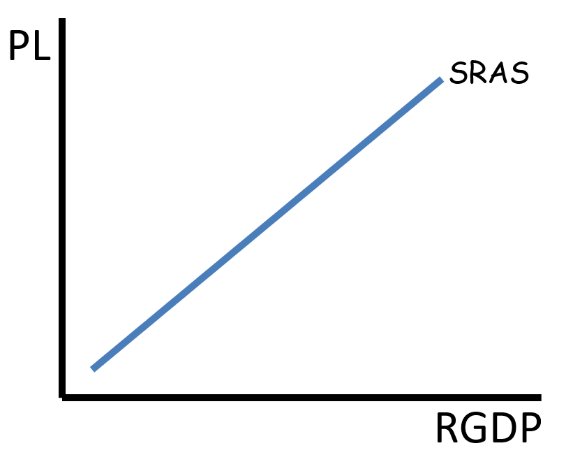
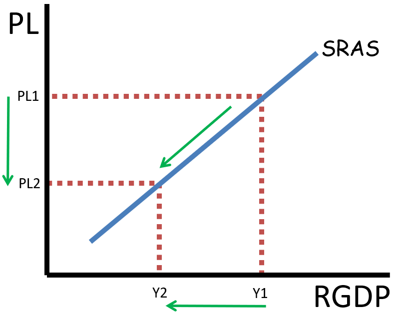
The short-run aggregates supply curve (SRAS) is upward sloping just like a typical market supply curve for an individual good or service. Instead of showing the direct relationship between the price and quantity of a product supplied within a market. The SRAS curve shows the direct relationship between the price level (on the y-axis) and the quantity of real GDP supplied (on the x-axis) in the short run. Since there is a direct relationship, that means there will be more goods and services supplied at higher price levels. And fewer goods and services supplied at lower price levels. This direct relationship exists in the short-run because wages and other resources prices are sticky in the short-run, meaning they are slow to adjust to higher or lower price levels. That means that when price levels rise, input costs generally stay low in the short run, so producers can earn higher profit margins by increasing production. Likewise, if price levels fall, input costs don’t change in the short run, so profit levels, causing producers to decrease production.

Price Level Decrease

Price Level Increase

• Key Characteristics:

  • Price level increases lead to higher GDP output due to sticky input prices (e.g., wages).

  • Price level decreases lead to lower GDP output because of the lag in changing input prices.

• Sticky Prices: Wages and input prices are "sticky," meaning they don't adjust quickly to changes in the price level. Producers can earn higher profits with increased production when prices rise in the short run, but will cut production when prices fall.

Summary (SRAS)

• Direct relationship between price level and real GDP in the short run.

• Sticky wages and prices create profit incentives to increase production as price levels rise.

• SRAS curve slopes upward.

Key Terms

• Short-Run Aggregate Supply (SRAS): Shows the direct relationship between price level and real GDP.

• Sticky Prices: Prices, especially wages, that are slow to adjust.

• Profitability: The incentive for firms to increase production when price levels rise.

Formula:

• No specific formula for SRAS, but the graph shows the positive correlation between price level and real GDP.

2. What are the SRAS Shifters?

Just like with aggregate demand, a change in the price level will not cause a change in aggregate demand. Changes in price level only cause movement up (with a price level increase) and or down (with a price level decrease) the SRAS curve. But there are things beside price level that cause producers throughout an economy to increase and decrease production, and when those things change, the SRAS curve will shift to the right (for an increase) or left (for a decrease).

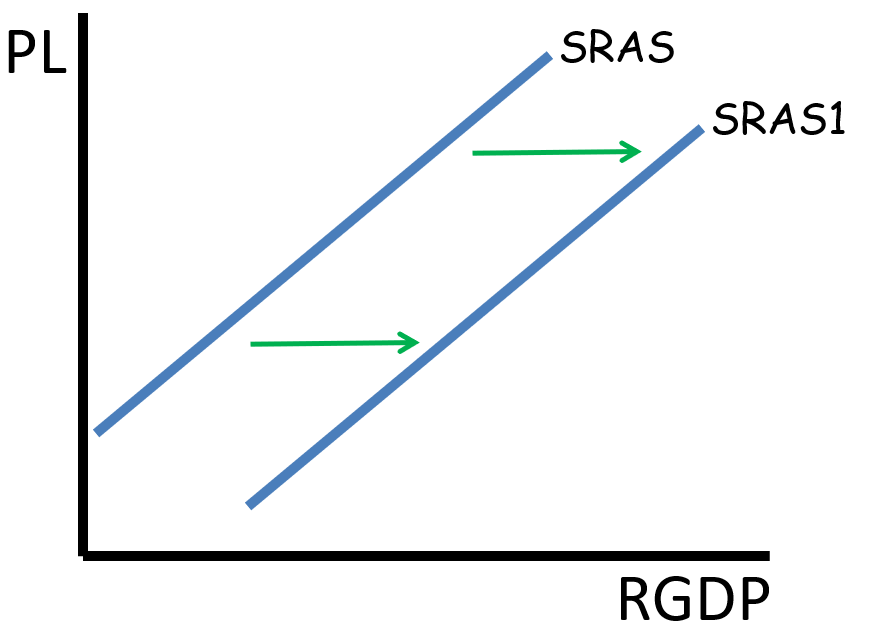
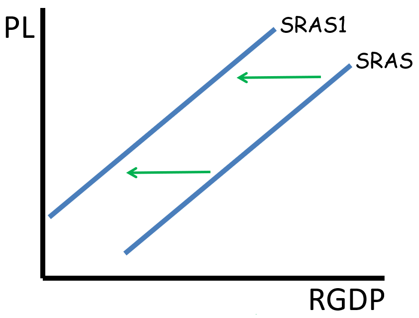
The first SRAS shifter is resource prices. Prices of major resources needed in the production of most goods (like wages, land, energy, etc.) have a direct impact on the profitability of producing most goods and services. When resource prices fall, profitability increases, so businesses produce more goods and services, shifting the SRAS curve to the right. When resource prices rise, profitability decreases, so businesses produce fewer goods and services, shifting the SRAS curve to the left.

SRAS Increase

SRAS Decrease

Changes in productivity can also shift the SRAS curve. When workers are able to produce more goods and services per hour of work (due to increases in human capital, the physical capital stock, technology improvements, etc), the SRAS curve will shift to the right. If there is a decrease in productivity, the SRAS curve will shift to the left.

If the government increases business regulations, the production costs generally increase. That reduces profitability causing businesses to reduce production, which shifts SRAS to the left. If, on the other hand, the government decreases business regulations, production costs can be expected to fall. Profitability will then increase, causing production throughout the economy to decrease, which shifts the SRAS curve shift to the right.

A decrease in taxes on businesses will cause the SRAS to increse (shift to the right), and an increase in taxes on businesses will cause the SRAS to decrease (shift to the left). 
Note: For the purposes of the AP exam, a change in taxes not specifically on businesses will shift the AD curve

The last SRAS shifter is changes in inflation expectations. When inflation expectations rise, resource prices begin to also rise (as workers demand high wages due to the higher expected inflation). Those higher resource prices cause a leftward shift of the SRAS. When inflation expectations decrease, the SRAS curve shifts right.

• Resource Prices: Changes in wages, land, energy, and other inputs can shift SRAS. Lower resource prices increase profitability and shift SRAS right, while higher resource prices shift it left.

• Productivity: An increase in productivity (e.g., through technology) shifts SRAS right, and a decrease shifts it left.

• Business Regulations: Less regulation reduces costs and shifts SRAS right, while more regulation increases costs and shifts SRAS left.

• Taxes on Businesses: Decreases in taxes shift SRAS right; increases in taxes shift SRAS left.

• Inflation Expectations: Higher inflation expectations push input prices up, shifting SRAS left. Lower inflation expectations shift SRAS right.

Summary (SRAS Shifters)

• Rightward shifts: Lower resource prices, higher productivity, deregulation, lower taxes, lower inflation expectations.

• Leftward shifts: Higher resource prices, lower productivity, more regulation, higher taxes, higher inflation expectations.

Key Terms

• Productivity: The efficiency with which goods and services are produced.

• Resource Prices: Costs associated with inputs like labor and raw materials.

• Business Regulations: Government rules impacting production costs.

3. What is Long-run Aggregate Supply?

Long-run aggregate supply (LRAS) shows that there is no relationship between the price level and real GDP output in the long run. At both high price levels and low-price levels, real GDP will always be equal to the full employment level of real GDP (Yf on the graph). This full employment level of output is equal to long-run potential real GDP from the business cycle graph. It is also the amount of real GDP an economy produces when there is no cyclical unemployment (only frictional and structural unemployment), and the unemployment rate is equal to the natural rate of unemployment.

The LRAS curve is vertical because wages and other resource prices are flexible (change to the new price level) in the long run. If price levels rise, and resource prices (like wages) also rise by the same amount (in the long run), then profitability doesn’t change, so businesses do not change their level of production. If price levels fall, then wages and other resource prices also fall by the same amount, profit ability will be constant, so businesses will again maintain their current level of production.

We will learn more about why it is that economies produce the full employment level of output in the long-run, when we learned about long-run adjustments in the AS/AD model.

• Definition: LRAS is vertical because, in the long run, real GDP remains constant at the full employment level, regardless of price level changes.

• Key Characteristics:

  • Wages and input prices are flexible in the long run.

  • Real GDP is fixed at full employment (Yf), unaffected by price changes.

  • The economy always returns to its potential output over time, even after economic shocks.

Summary (LRAS)

• Vertical LRAS curve shows that long-run real GDP is independent of price level.

• Full employment GDP is achieved when cyclical unemployment is zero.

• Price level changes do not affect GDP in the long run.

Key Terms

• Long-Run Aggregate Supply (LRAS): A vertical line representing the full employment level of GDP.

• Full Employment: The level of GDP where there is no cyclical unemployment.

4. What are the Long-run Aggregate Supply Shifters?

Since the LRAS is vertical at an economy’s long-run potential real GDP, the LRAS will shift right when potential GDP increases, and left when potential GDP decreases. As a result, it may be helpful to think about the LRAS curve as being similar to the production possibilities curve (PPC). Anything that would shift the PPC outward, will shift the LRAS curve to the right. Anything that would shift the PPC inward, will shift the LRAS curve to the left.

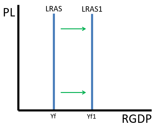
LRAS Increase

LRAS Decrease

Changes in the quantity of resources is the first of our LRAS shifters. When there are more resources available, the LRAS will shift to the right, and when there are fewer resources available, the LRAS will shift to the left.

The second LRAS shifter is the quality of resources. When workers get more productive through improvements in human capital (skills and knowledge of workers), potential real GDP increases, shifting the LRAS to the right. If workers become less knowledgeable and skilled, the LRAS will shift to the left.

The last of the LRAS shifters is Productivity of resources. Technology changes, or changes in the amount of physical capital (called the capital stock), will change productivity. More productivity will shift the LRAS to the right, and less productivity will shift the LRAS to the left.

• Quantity of Resources: More resources (e.g., labor, capital) shift LRAS right, and fewer resources shift it left.

• Quality of Resources: Better educated and skilled workers shift LRAS right. Lower quality resources shift LRAS left.

• Productivity: Technological advancements and capital investment increase productivity, shifting LRAS right.

Summary (LRAS Shifters)

• Rightward shifts: Increases in resources, better quality resources, higher productivity.

• Leftward shifts: Decreases in resources, lower quality resources, lower productivity.

Key Terms

• Resource Quantity: The total amount of labor, capital, and natural resources available.

• Productivity of Resources: Efficiency of inputs like labor and technology in producing goods.