
 Worksheets
Numerical Descriptive Measures
Total questions: 124
Worksheet time: 1hrs 11mins
is the extent to which all the data values group around a typical or central value
(a)
is the amount of dispersion of scattering of values
(a)
is the pattern of the distribution of values from the lowest value to the highest value.
(a)
is the most common measure of central tendency
(a)
X̄
(a)
n
(a)
Xi
(a)
sum of values divided by the number of values
(a)
Mean is affected by extreme values (outliers)
True
False
is the “middle” number (50% above, 50% below)
mean
median
mode
Median is not affected by extreme values
True
False
The location of the median when the values are in numerical order (smallest to largest)
True
False
If the number of values is odd, the median is the middle number
True
False
If the number of values is even, the median is the average of the two middle numbers
True
False
Note that (a) is not the value of the median, only the position of the median in the ranked data
value that occurs most often
(a)
Mode is not affected by extreme outliers
True
False
used for either numerical or categorical (nominal data)
(a)
In mode, there may be no (a)
In mode, there may be several (a)
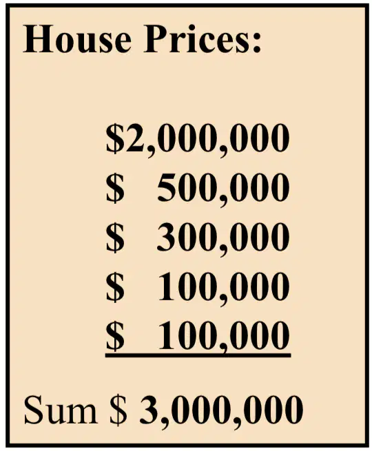
Compute the Mean
(a)
Get the Mode
(a)
middle value of ranked data
mean
mode
median
most frequent value
median
mode
mean
is generally used, unless extreme values (outliers) exist.
median
mean
mode
is often used, since the it is not sensitive to extreme values.
mode
mean
median
In some situations, it makes sense to report both the _____ and the ______.
mean and mode
mode and median
mean and median
ratio interval
mean
median
mode
Ratio Interval Ordinal
mean
median
mode
Ratio Interval Ordinal Nominal
mean
median
mode
numerical center of the data
mean
median
mode
Sum of deviations from the mean is zero
mean
median
mode
Computed only from the center values
mean
median
mode
Sensitive to extreme values
mean
median
mode
Not sensitive to extreme values
mean
median
mode
Does not use information from all the data
mean
median
mode
May not reflect the center
mean
median
mode
May not exist
mean
median
mode
Might have multiple modes
mean
median
mode
give information on the spread or variability or dispersion of the data values.
measures of variation
measures of variablity
measures of variable
measures of dispersion
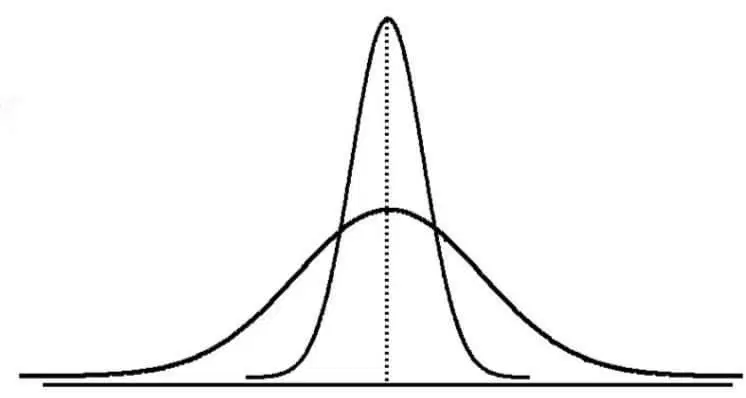
Describe the picture
same variation and center
same variation, different center
same center, different variation
different variation and center
Simplest measure of variation
mode
variance
range
standard deviation
No causal effect is implied
mode
variance
range
standard deviation
Difference between the largest and the smallest values
mode
variance
range
standard deviation
Only concerned with the strength of the relationship
mode
covariance
range
standard deviation
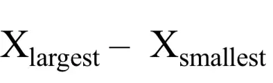
How to compute range?
Xlargest - Xsmallest
Xlargest + Xsmallest
Xsmallest - Xlargest
Xsmallest / Xlargest
Why the range can be misleading?
Not sensitive to outliers
Ignores the way in which data are distributed
Sensitive to outliers
Both B and C
average (approximately) of squared deviations of values from the mean
The Coefficient of Variance
The Sample Variance
The Sample Variable
The Sample Variablity
Formula of sample variance

Formula of sample covariance

Formula of z-score

most commonly used measure of variation
variance
range
standard deviation
mean
shows variation about the mean
mean
median
variance
standard deviation
is the square root of the variance
mean
median
variance
standard deviation
has the same units as the original data
mean
median
variance
standard deviation
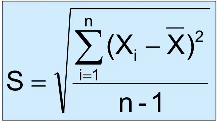
Formula of sample standard deviation
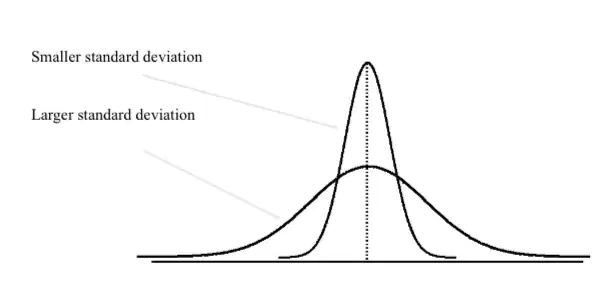
Describe the image
The more the data are spread out, the greater the range, variance, and standard deviation.
The more the data are concentrated, the smaller the range, variance, and standard deviation.
If the values are all the same (no variation), all these measures will be zero.
All of the above
Measures relative variation
The Coefficient of Variable
The Coefficient of Variance
The Coefficient of Variation
The Coefficient of Variability
Always in percentage (%)
The Coefficient of Variable
The Coefficient of Variance
The Coefficient of Variation
The Coefficient of Variability
Shows variation relative to mean
The Coefficient of Variable
The Coefficient of Variance
The Coefficient of Variation
The Coefficient of Variability
Can be used to compare the variablity of two or more sets of data measured in different units
The Coefficient of Variable
The Coefficient of Variance
The Coefficient of Variation
The Coefficient of Variability
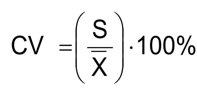
Formula of coefficients of variation
To compute the _____ of a data value, subtract the mean and divide
by the standard deviation.
z-score
range
median
variance
measures the strength of the linear relationship between
two numerical variables (X & Y)
z-score
range
median
covariance
A data value is considered an extreme outlier if its Z-score is less
than _____ or greater than _____.
-3.0, +3.0
+3.0, -3.0
-2.0, +3.0
-3.0, +2.0
The larger the absolute value of the Z-score, the farther the data
value is from the mean.
False
Maybe
True
Yes
Suppose the mean math SAT score is 490, with a standard deviation of 100. Compute the Z-score for a test score of 620.
1.6
1.4
1.2
1.3
Measures the amount of asymmetry in a distribution
Kurtosis
Skewness
Weighted Mean
Percentile
A tool that is helpful in describing data in certain circumstances is
called the _____
Kurtosis
Empirical Rule
Weighted Mean
Percentile
is approximates the variation of data in a bell-shaped distribution
Kurtosis
Empirical Rule
Weighted Mean
Percentile
In Empirical Rule, approximately _____ of the data in a bell shaped distribution is within ± one
standard deviation of the mean or
-69%
70%
68%
69%
Measures the relative concentration of values in the center of
a distribution as compared with the tails
Kurtosis
Skewness
Weighted Mean
Percentile
split the ranked data into 4 segments with an equal
number of values per segment
Kurtosis
Skewness
Weighted Mean
Quartiles
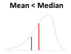
Describe the shape of Skewness
Symmetric
Right-Skewed
Left-Skewed
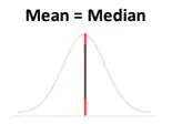
Describe the shape of Skewness
Symmetric
Right-Skewed
Left-Skewed
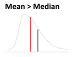
Describe the shape of Skewness
Symmetric
Right-Skewed
Left-Skewed

Describe the shape of Kurtosis
Sharper Peak
Than Bell-Shaped
Flatter Than
Bell-Shaped
Bell-Shaped
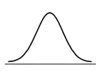
Describe the shape of Kurtosis
Sharper Peak
Than Bell-Shaped
Flatter Than
Bell-Shaped
Bell-Shaped

Describe the shape of Kurtosis
Sharper Peak
Than Bell-Shaped
Flatter Than
Bell-Shaped
Bell-Shaped
Formula of Weighted Mean for a Population
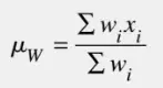
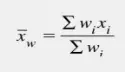

Bell-Shaped
Formula of Weighted Mean for a Sample
Bell-Shaped
Formula of Sample Coefficient of Correlation
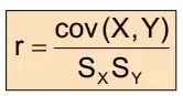
Bell-Shaped
Formula of Percentile
Bell-Shaped
Formula of Quartiles
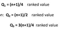
Bell-Shaped

Myers & Associates Recently, the law firm of Myers & Associates was involved in litigating a discrimination suit concerning ski instructors at a ski resort in Colorado. One ski instructor from Germany had sued the operator of the ski resort, claiming he had not received equitable pay compared with the other ski instructors from Norway and the United States. In preparing a defense, the Myers attorneys planned to compute the mean annual income for all seven Norwegian ski instructors at the resort. However, because these instructors worked different numbers of days during the ski season, a weighted mean needed to be computed. The following data and weights were determined:
$5,558.52
$5,456.52
$5,668.52
$5,568.52
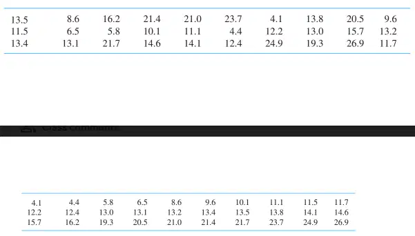
The Henson Trucking Company is a small company in the business of moving people
from one home to another within the Dallas, Texas, area. Historically, the owners have
charged the customers on an hourly basis, regardless of the distance of the move within
the Dallas city limits. However, they are now considering adding a surcharge for moves
over a certain distance. They have decided to base this charge on the 80th percentile.
They have a sample of travel-distance data for 30 moves. These data are as follows:
23
24
25
26
The first quartile, Q1, is the value for which 25% of the observations
are smaller and 75% are larger
True
False
Q2 is the same as the median (50% of the observations are smaller
and 50% are larger)
True
False
Only 25% of the observations are greater than the third quartile
True
False
is Q3 – Q1 and measures the spread in the middle 50% of the
data
Quartile
Percentile
Weighted Mean
Interquartile Range (IQR)
is also called the midspread because it covers the middle 50%
of the data
Quartile
Percentile
Weighted Mean
Interquartile Range (IQR)
is a measure of variability that is not influenced by outliers or
extreme values
Quartile
Percentile
Weighted Mean
Interquartile Range (IQR)
A Graphical display of the data based on the five-number summary
Quartile
Boxplot
Weighted Mean
Interquartile Range (IQR)
can be shown in either a vertical or horizontal orientation
Quartile
Boxplot
Weighted Mean
Interquartile Range (IQR)
Measures like Q1, Q3, and IQR that are not influenced by outliers are
called
resistant measures
resistant variable
resistant quartiles
resistant IQR and quartiles
Solving for IQR: Any number greater than this is an outlier
Q3 + (1.5 x IQR)
Q3 + (1.4 x IQR)
Q3 + (1.3 x IQR)
Q3 + (1.2 x IQR)
Solving for IQR: Any number less than this is an outlier.
Q1 – (1.5 x IQR)
Q1 – (1.4 x IQR)
Q1 – (1.3 x IQR)
Q1 – (1.2 x IQR)
The five numbers that help describe the center,
spread and shape of data are:
• Xsmaller
• First Quartile (Q1)
• Median (Q2)
• Third Quartile (Q3)
• Xlarger
• Xlarge
• First Quartile (Q1)
• Median (Q2)
• Third Quartile (Q3)
• Xsmall
• Xsmallest
• First Quartile (Q1)
• Median (Q2)
• Third Quartile (Q3)
• Xlargest
• Xsmallest
• First Quartile (Q2)
• Median (Q1)
• Third Quartile (Q3)
• Xlargest
Relationships among the five-number summary and
distribution shape
Median – Xsmallest > Xlargest – Median
Q1 – Xsmallest > Xlargest – Q3
Median – Q1 >Q3 – Median
Right-Skewed
Left-Skewed
Symmetric
Relationships among the five-number summary and
distribution shape
Median – Xsmallest ≈ Xlargest – Median
Q1 – Xsmallest ≈ Xlargest – Q3
Median – Q1 ≈ Q3 – Median
Right-Skewed
Left-Skewed
Symmetric
Relationships among the five-number summary and
distribution shape
Median – Xsmallest < Xlargest – Median
Q1 – Xsmallest < Xlargest – Q3
Median – Q1 < Q3 – Median
Right-Skewed
Left-Skewed
Symmetric
Shape of Boxplots: If data are symmetric around the median then the box and central line are
centered between the endpoints
True
False
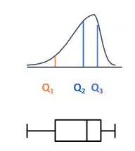
Determine the shape of distribution and the box plot
Left-Skewed
Symmetric
Right-Skewed

Determine the shape of distribution and the box plot
Left-Skewed
Symmetric
Right-Skewed
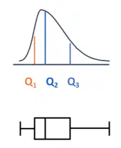
Determine the shape of distribution and the box plot
Left-Skewed
Symmetric
Right-Skewed
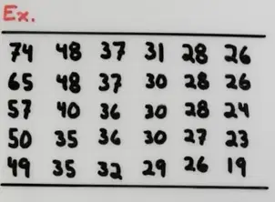
A manufacturer of insulation randomly selects 20 winter days and records the daily high temperature
24, 35, 17, 21, 24, 37, 26, 46, 58, 30, 32, 13, 12, 38, 41, 43, 44, 27, 53, 27
Find the mean and the five-number summary
Mean: 33.4
Five Number Summary
Xsmallest = 13
Q1 = 24
Q2 = 31
Q3 = 41.5
Xlargest = 60
Mean: 32.6
Five Number Summary
Xsmallest = 12
Q1 = 24
Q2 = 32
Q3 = 41.5
Xlargest = 78
Mean: 32.4
Five Number Summary
Xsmallest = 12
Q1 = 25
Q2 = 31
Q3 = 41.8
Xlargest = 90
Mean: 32.4
Five Number Summary
Xsmallest = 12
Q1 = 24
Q2 = 31
Q3 = 41.5
Xlargest = 58
The following list displays the scores of the latest test in Ben Faire’s algebra class.
83 76 82 62 57 82 83 72 76 74 90 84. Find the standard deviation and variance.
Standard Deviation = 9.54
Variance = 90.93
Standard Deviation = 10.54
Variance = 91.93
Standard Deviation = 9.60
Variance = 92.93
Standard Deviation = 9.54
Variance = 43.93
Grades on a history exam follow a normal distribution with a mean of 78 and a standard deviation 6. Find the range around the mean that includes 95% of the grades. Use the Empirical Rule formula
66 & 90
68 & 91
65 & 90
57 & 85
The heights of women follow a bell-shaped distribution with a mean of 160 cm and a standard deviation of 7.5 cm. What is the approximate percentage of women between 137.5 cm and 182.5 cm. Use the Empirical Rule formula.
6
4
5
3
Regardless of how the data are distributed, at least (1 - 1/k2) x
100% of the values will fall within k standard deviations of the
mean (for k > 1)
Empirical Rule
Chebyshev Rule
Your Rule
Variance Rule
What proportion of the data is within 2 standard deviation of the mean?
7.5 & 68.7
11.5 & 60.7
10.5 & 61.7
9.6 & 70.7
The average price of a new car is $36,000, with a standard deviation of $4,100. What is the main percentage of card that should sell between $22,000 and $50,000?
96.3%
90.3%
94.3%
91.3%
It is not possible to determine the relative strength of the relationship
from the size of the covariance
True
False
X and Y tend to move in the same direction
cov(X,Y) < 0
cov(X,Y) > 0
cov(X,Y) = 0
X and Y tend to move in opposite directions
cov(X,Y) < 0
cov(X,Y) > 0
cov(X,Y) = 0
X and Y are independent
cov(X,Y) < 0
cov(X,Y) > 0
cov(X,Y) = 0
Measures the relative strength of the linear relationship between two
numerical variables
Coefficient of Condensation
Coefficient of Concentation
Coefficient of Correlation
Coefficient of Corresponding
The closer to –1, the weaker the negative linear relationship
True
False
The closer to 1, the stronger the positive linear relationship
True
False
The closer to 0, the stronger the linear relationship
True
False
Data analysis is objective
False
True
Should report the summary measures that best
describe and communicate the important aspects of
the data set
False
True
Data interpretation is subjective
False
True
Should be done in fair, neutral and clear manner
False
True